Precision And Recall

Precision and recall are metrics used to describe the performance of binary predictors.

Terminology Note

Precision and Recall are used extensively in Inforation retreival. In this context,

relevant document = true instance
retrieved document = true prediction

Precision¶

Given a set of True / False predictions and corresponding True / False instances, precision represents the accuracy rate of True predictions. It is sometimes referred to as positive prediction value.

Formula¶

\[ \text{Precision} =\frac{\text{True Positives}}{\text{True Positives} + \text{False Positives}} \]

Example¶

|pred  |truth |
|:-----|:-----|
|True  |True  |  <- true positive
|True  |True  |  <- true positive
|False |True  |
|False |True  |
|False |False |
|True  |False |  <- false positive
|False |False |
|False |False |

\(\text{True Positives} = 2\)
\(\text{False Positives} = 1\)

\[ \text{Precision} = \frac{\text{2}}{\text{2} + \text{1}} = 0.67 \]

Recall¶

Given a set of True/False predictions and corresponding True/False instances, recall represents the accuracy rate of predictions on True instances. It is sometimes referred to as sensitivity.

Formula¶

\[ \text{Recall} = \frac{\text{True Positives}}{\text{True Positives} + \text{False Negatives}} \]

Example¶

|pred  |truth |
|:-----|:-----|
|True  |True  |  <- true positive
|True  |True  |  <- true positive
|False |True  |  <- false negative
|False |True  |  <- false negative
|False |False |
|True  |False |
|False |False |
|False |False |

\(\text{True Positives} = 2\)
\(\text{False Negatives} = 2\)

\[ \text{Recall} = \frac{\text{2}}{\text{2} + \text{2}} = 0.5 \]

F-Score¶

F-Score combines precision and recall into a single score in the range [0, 1], where

0 indicates that all positive predictions are incorrect
1 indicates that all true instances are correctly predicted with zero false positives

Formula¶

F₁ Score (Balanced F-Score)

Here, precision and recall are considered equally important.

\[ F_{1}={\frac {2}{\mathrm {\frac{1}{precision}} + \mathrm {\frac{1}{recall}}}}= 2\cdot {\frac {\mathrm {precision} \cdot \mathrm {recall} }{\mathrm {precision} +\mathrm {recall} }} \]

F_BScore (Generalized F-Score)

Here, recall is considered \(\beta\) times as important as precision.

\[ F_\beta = (1 + \beta^2) \cdot \frac{\mathrm{precision} \cdot \mathrm{recall}}{(\beta^2 \cdot \mathrm{precision}) + \mathrm{recall}} \]

Example¶

Calculate F_0.5, F₁, and F₂ for the following data.

|pred  |truth |
|:-----|:-----|
|True  |True  |
|True  |True  |
|False |True  |
|False |True  |
|False |False |
|True  |False |
|False |False |
|False |False |

\(\text{precision} = 0.67\)
\(\text{recall} = 0.50\)

\[ F_{0.5} = (1 + 0.5^2) \cdot {\frac {0.67 \cdot 0.5}{(0.5^2 \cdot 0.67 + 0.50)}} = .63 \]

\[ F_1 = {\frac {2 \cdot 0.67 \cdot 0.5}{(0.67 + 0.50)}} = 0.57 \]

\[ F_2 = (1 + 2^2) \cdot {\frac {0.67 \cdot 0.5}{(2^2 \cdot 0.67 + 0.50)}} = 0.53 \]

Precision-Recall Curve¶

The Precision-Recall Curve plots precision vs recall for a range of classification thresholds. For example, suppose we have the following predicted scores and truths.

| pred_score | truth |
|:----------:|:-----:|
|   0.349    | True  |
|   -1.084   | False |
|   -0.270   | False |
|   0.360    | True  |
|   0.898    | True  |
|   -1.923   | True  |
|   0.552    | True  |
|   -2.273   | False |
|   -1.986   | False |
|   -0.122   | True  |
|   -1.738   | False |
|   -3.082   | False |

If we assume a classification threshold of 0 (also known as a cutoff value), we can convert each prediction score to a prediction class.

\(\text{pred_class} = \text{pred_score} \ge 0\)

| pred_score | pred_class | truth |
|:----------:|:----------:|:-----:|
|   0.349    |    True    | True  |
|   -1.084   |   False    | False |
|   -0.270   |   False    | False |
|   0.360    |    True    | True  |
|   0.898    |    True    | True  |
|   -1.923   |   False    | True  |
|   0.552    |    True    | True  |
|   -2.273   |   False    | False |
|   -1.986   |   False    | False |
|   -0.122   |   False    | True  |
|   -1.738   |   False    | False |
|   -3.082   |   False    | False |

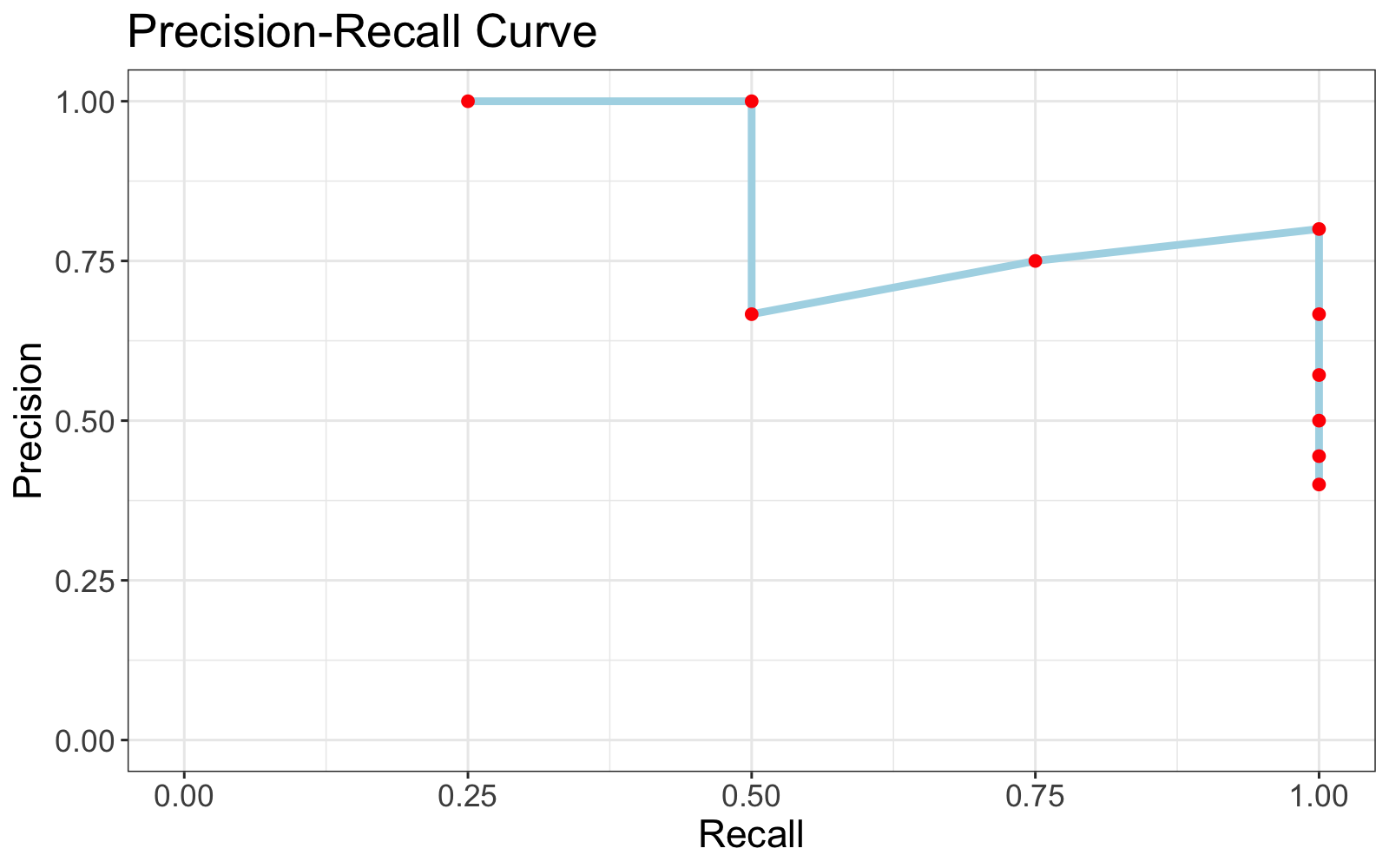
Here, recall = 0.67 and precision = 1.00. This pair of values, (0.67, 1.00), is one point on the Precision-Recall curve. Repeating this process for a range of classification thresholds, we can produce a Precision-Recall curve like the one below.

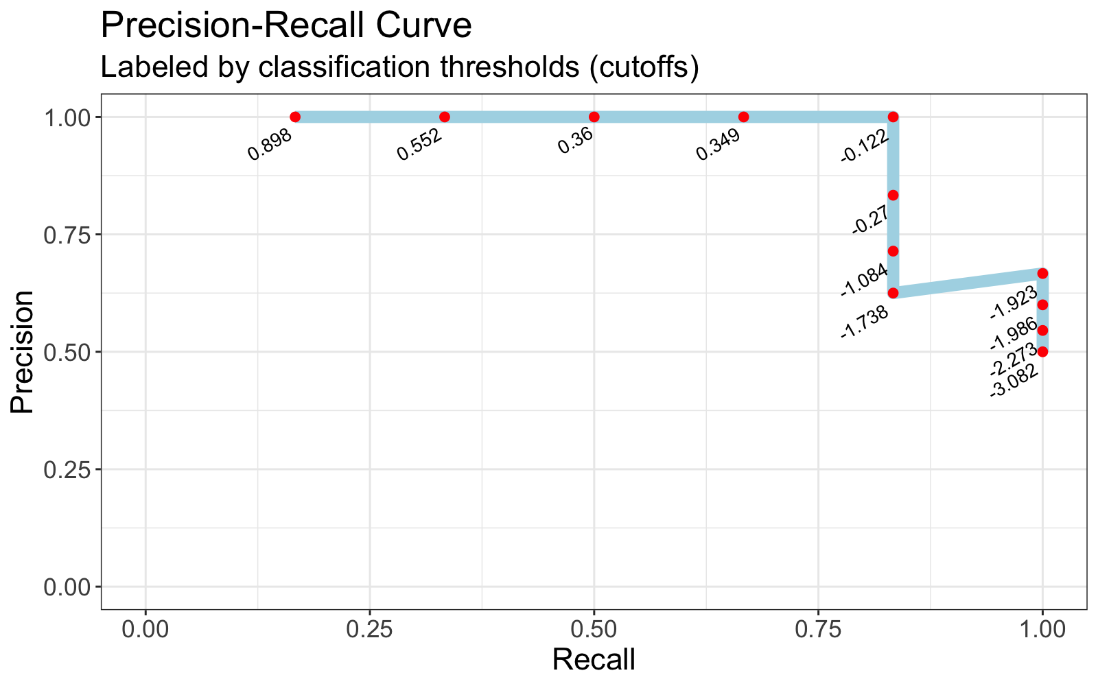
Plot data

| threshold | precision | recall |
|:---------:|:---------:|:------:|
|   0.898   |   1.00    |  0.17  |
|   0.552   |   1.00    |  0.33  |
|   0.360   |   1.00    |  0.50  |
|   0.349   |   1.00    |  0.67  |
|  -0.122   |   1.00    |  0.83  |
|  -0.270   |   0.83    |  0.83  |
|  -1.084   |   0.71    |  0.83  |
|  -1.738   |   0.62    |  0.83  |
|  -1.923   |   0.67    |  1.00  |
|  -1.986   |   0.60    |  1.00  |
|  -2.273   |   0.55    |  1.00  |
|  -3.082   |   0.50    |  1.00  |

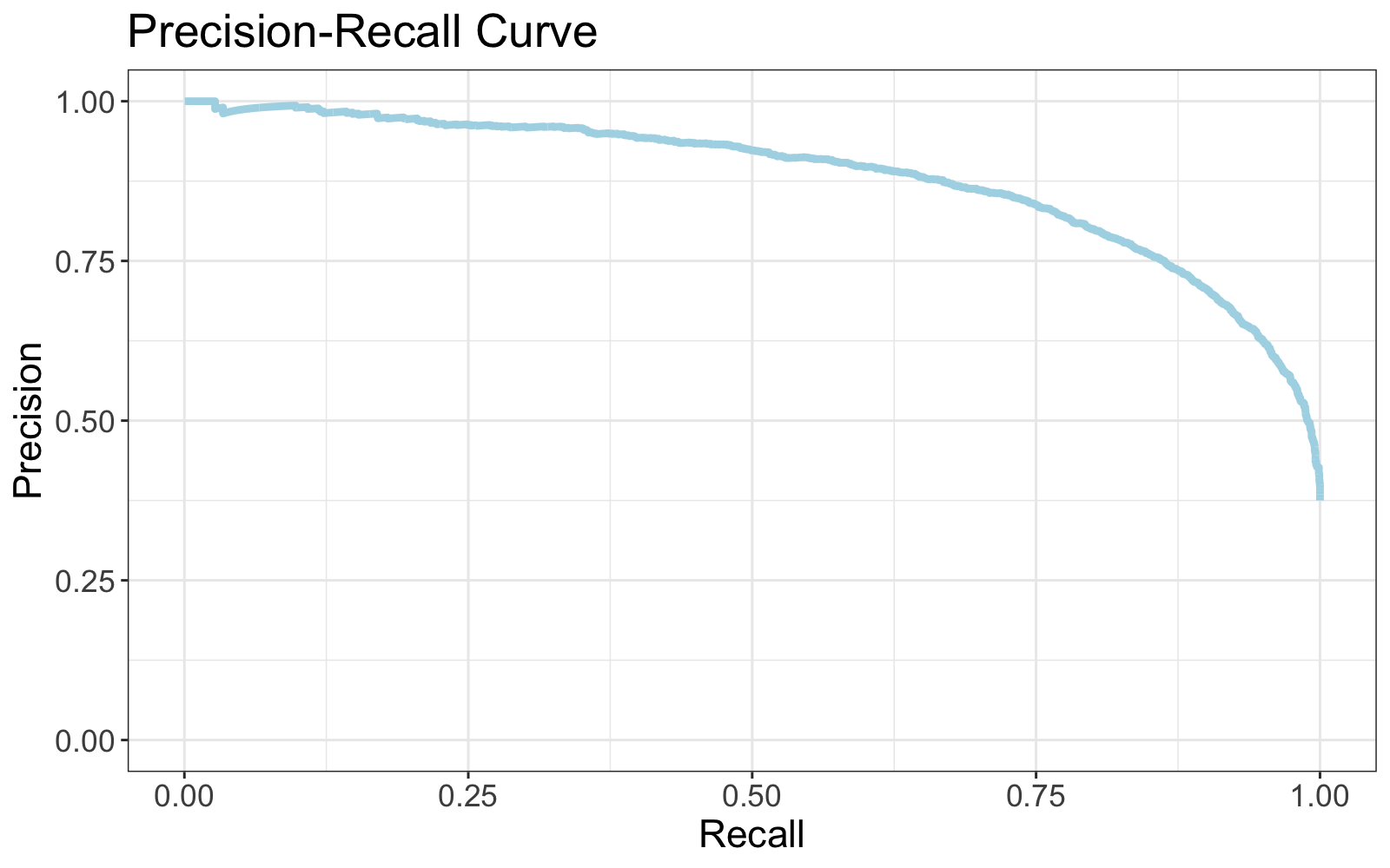
It doesn't look much like a curve in this tiny example, but Precision-Recall curves applied to larger data usually look more like this.

R code to reproduce this plot

library(data.table)
library(ggplot2)

trues <- rnorm(3000)
falses <- rnorm(5000, -2)

dt <- data.table(
  pred_score = round(c(trues, falses), 3),
  truth = c(rep(T, length(trues)), rep(F, length(falses)))
)

# sort the data from highest likelihood of True to lowest likelihood of True
setorderv(dt, "pred_score", order = -1)

# calculate Precision and Recall for each threshold
# (we predict true where score >= threshold)
dt[, `:=`(
  TP = cumsum(truth == T),
  FP = cumsum(truth == F),
  FN = c(tail(rev(cumsum(rev(truth))), -1), 0)
)]
dt[, `:=`(
  precision = TP/(TP + FP),
  recall = TP/(TP + FN)
)]

ggplot(dt, aes(x = recall, y = precision))+
  geom_line(size = 1.5, color = "light blue")+
  labs(x = "Recall", y = "Precision", title = "Precision-Recall Curve")+
  ylim(0,1)+
  xlim(0,1)+
  theme_bw()+
  theme(text = element_text(size=16))

Note

Precision generally decreases as recall increases, but this relationship is not guaranteed.

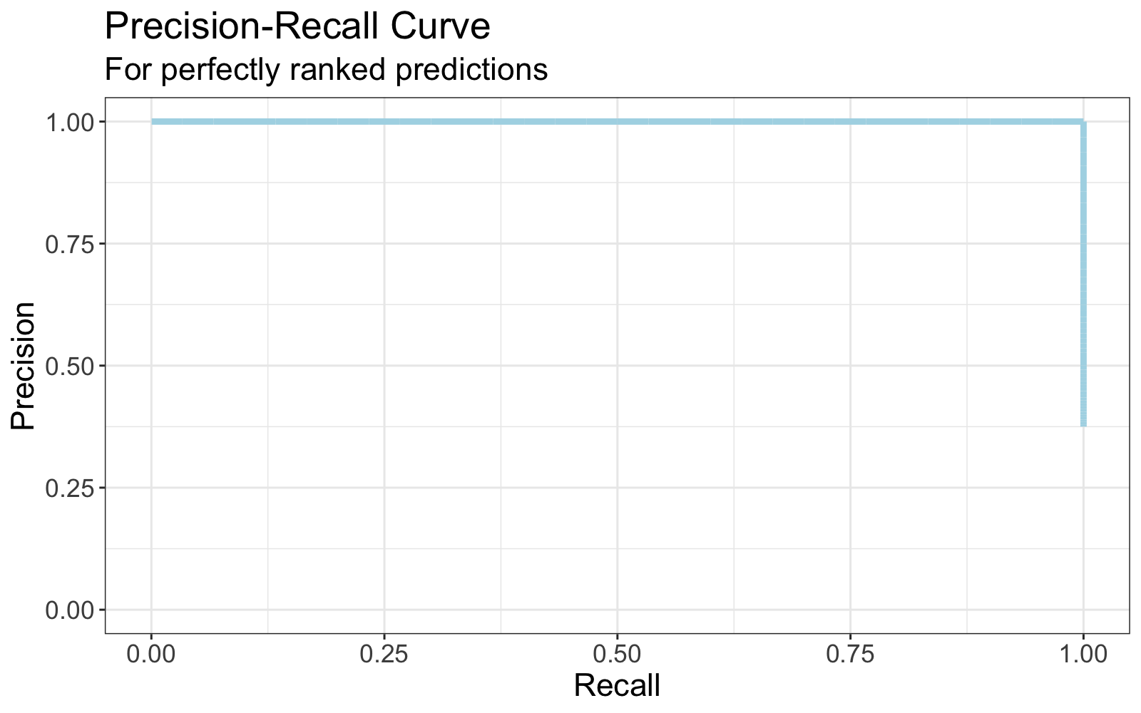
Perfectly ranked prediction scores are reflected by a Precision-Recall curve like this.

Average Precision¶

Consider predictions from two models A & B compared to known thruths.

| preds_A | preds_B | truths |
|:-------:|:-------:|:------:|
|  True   |  True   |  True  |
|  True   |  True   |  True  |
|  True   |  True   | False  |
|  True   |  True   | False  |
|  False  |  False  |  True  |
|  False  |  False  |  True  |
|  False  |  False  | False  |
|  False  |  False  | False  |

A and B have identical prediction classes, and therefore have identical precision, recall, and F-scores. However, suppose we reveal A's and B's prediction scores (in this case, probabilities).

| scores_A | scores_B | truths |
|:--------:|:--------:|:------:|
|   0.95   |   0.55   |  True  |  <- A & B are correct,   only A is confident
|   0.85   |   0.59   |  True  |  <- A & B are correct,   only A is confident
|   0.73   |   0.88   | False  |  <- A & B are incorrect, only B is confident
|   0.62   |   0.97   | False  |  <- A & B are incorrect, only B is confident
|   0.48   |   0.20   |  True  |  <- A & B are incorrect, only B is confident
|   0.39   |   0.09   |  True  |  <- A & B are incorrect, only B is confident
|   0.12   |   0.43   | False  |  <- A & B are correct,   only A is confident
|   0.04   |   0.32   | False  |  <- A & B are correct,   only A is confident

The classification threshold in this example is 0.5. That is, preds_A = scores_A >= 0.5 and preds_B = scores_B >= 0.5.

Observe

When model A was confident in its predictions, it was correct.
When model B was confident in its predictions, it was incorrect.

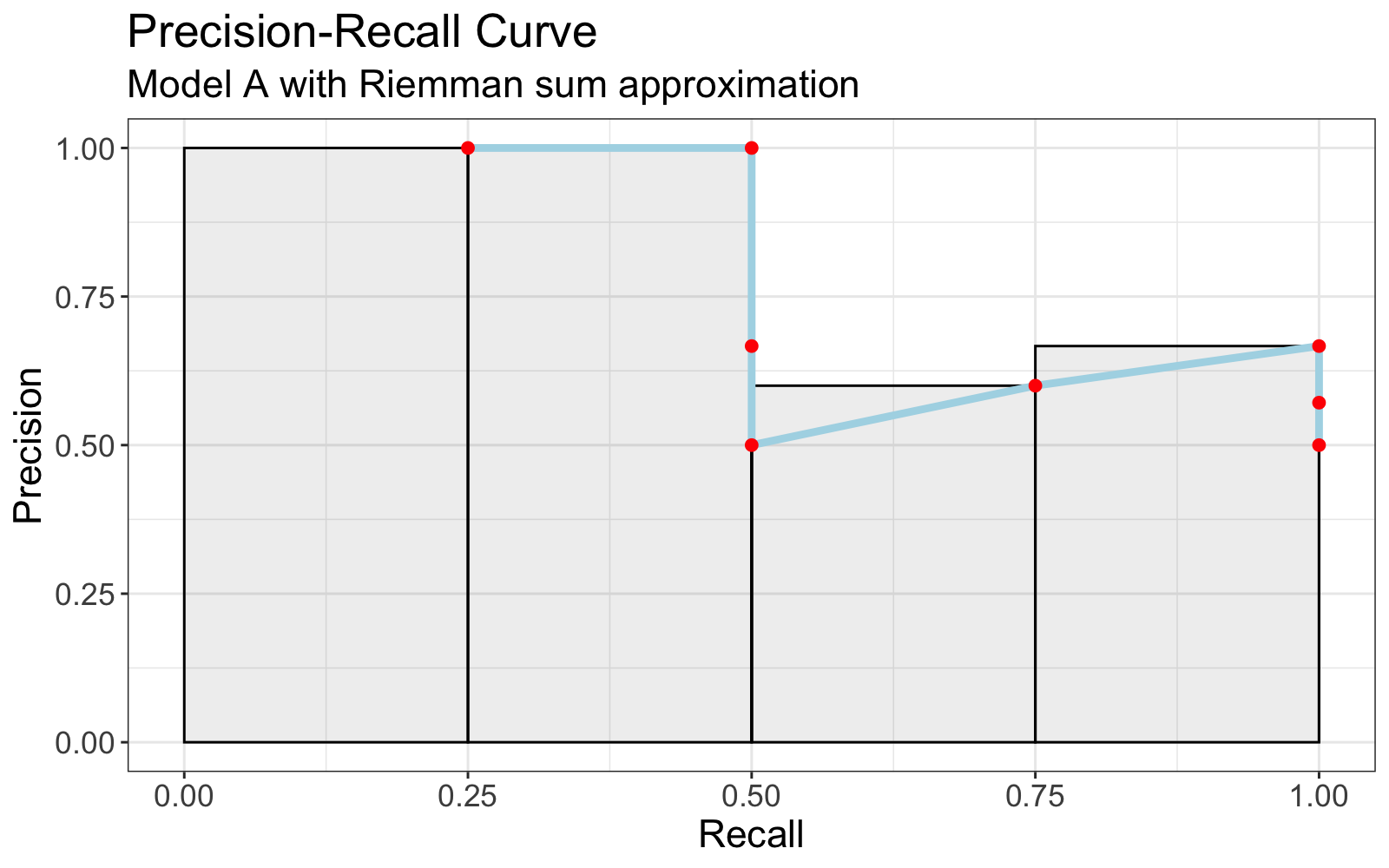
Intuitively, this suggests model A better than model B. This is depicted visually observing that A's Precision-Recall curve is consistently higher than B's Precision-Recall curve.

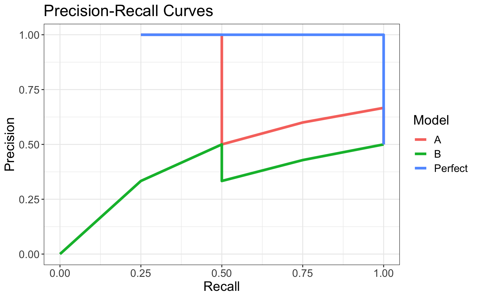
This desire to score ranked predictions leads to Average Precision which measures the average precision value on the Precision-Recall curve over the range [0, 1].

Formula¶

Average Precision equals area under the Precision-Recall curve.

\[ \operatorname{AveP} = \int_0^1 p(r)dr \]

where \(p(r)\) is the precision at recall \(r\).

This integral can be discretized as

\[ \operatorname{AveP} = \sum_{k=1}^n P(k) \Delta r(k) \]

where \(k\) is the rank in the sequence of prediction scores (high to low), \(n\) is the total number of samples, \(P(k)\) is the precision at cut-off \(k\) in the list, and \(\Delta r(k)\) is the change in recall from items \(k-1\) to \(k\).

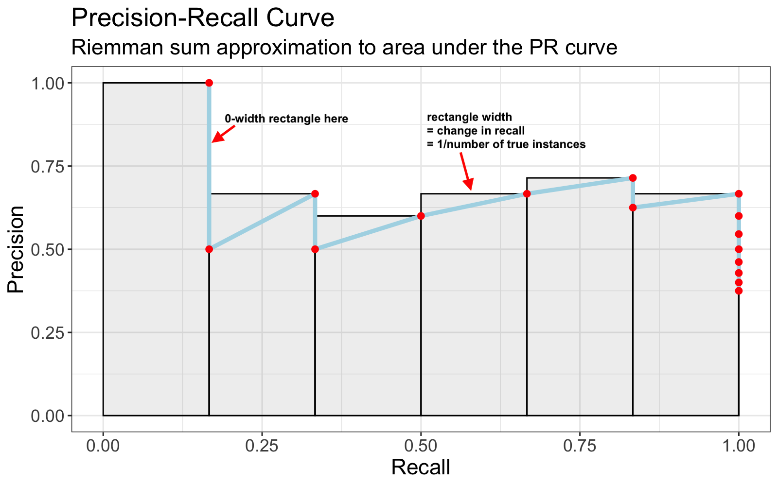
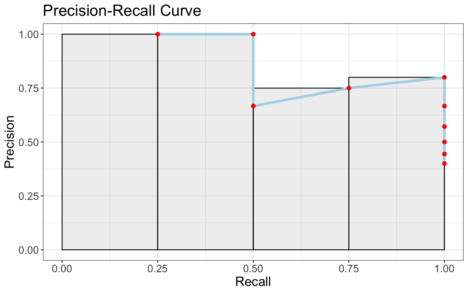
Geometrically, this formula represents a Riemann Sum approximation to the Precision-Recall curve using rectangles with height \(P(k)\) and width \(\Delta r(k)\).

R code to reproduce this plot

library(data.table)
library(ggplot2)

set.seed(4)
trues <- rnorm(6)
falses <- rnorm(10, -1)
dt <- data.table(
  pred_score = round(c(trues, falses), 3),
  truth = c(rep(T, length(trues)), rep(F, length(falses)))
)
setorderv(dt, "pred_score", order = -1)
dt[, `:=`(
  TP = cumsum(truth == T),
  FP = cumsum(truth == F),
  FN = c(tail(rev(cumsum(rev(truth))), -1), 0)
)]
dt[, `:=`(
  precision = TP/(TP + FP),
  recall = TP/(TP + FN)
)]
dt[, recall_prev := shift(recall, type = "lag", fill = 0)]
ggplot(dt, aes(x = recall, y = precision))+
  geom_rect(aes(xmin = recall_prev, xmax = recall, ymin = 0, ymax = precision), alpha = 0.1, color = "black")+
  geom_line(size = 1.5, color = "light blue")+
  geom_point(size = 2, color = "red")+
  labs(x = "Recall", y = "Precision", title = "Precision-Recall Curve", subtitle = "Riemman sum approximation to area under the PR curve")+
  ylim(0,1)+
  xlim(0,1)+
  theme_bw()+
  theme(text = element_text(size=16))

Since recall ranges from 0 to 1, this can be interpreted as a weighted sum of Precisions whose weights are the widths of the rectangles (i.e. the changes in recall from threshold to threshold), hence the name Average Precision.

Furthermore, the width of each non-zero-width rectangle is the same. Alternatively stated, each positive change in recall is equivalent. Thus, Average Precision can be described as an arithmetic mean of Precision values restricted to the set of True instances (relevant documents).

\[ \operatorname {AveP} ={\frac {\sum _{k=1}^{n}P(k)\times \operatorname {rel} (k)}{\mbox{number of true instances}}} \]

where \(\operatorname {rel} (k)\) is an indicator function equaling 1 if the item at rank \(k\) is a true instance, 0 otherwise.

Example¶

Using the toy data above,

Model AModel B

| scores_A | truths | precision_k | delta_recall_k | rel_k |
|:--------:|:------:|:-----------:|:--------------:|:-----:|
|   0.95   |  TRUE  |    1.00     |      0.25      |   1   | <- include
|   0.85   |  TRUE  |    1.00     |      0.25      |   1   | <- include
|   0.73   | FALSE  |    0.67     |      0.00      |   0   |
|   0.62   | FALSE  |    0.50     |      0.00      |   0   |
|   0.48   |  TRUE  |    0.60     |      0.25      |   1   | <- include
|   0.39   |  TRUE  |    0.67     |      0.25      |   1   | <- include
|   0.12   | FALSE  |    0.57     |      0.00      |   0   |
|   0.04   | FALSE  |    0.50     |      0.00      |   0   |

Formula 1

\[ \operatorname{AveP} = \sum_{k=1}^n P(k) \Delta r(k) = 1.00 \cdot 0.25 + 1.00 \cdot 0.25 + 0.60 \cdot 0.25 + 0.67 \cdot 0.25 = 0.82 \]

Formula 2

\[ \operatorname {AveP} ={\frac {\sum _{k=1}^{n}P(k)\times \operatorname {rel} (k)}{\mbox{number of true instances}}} = \frac{1.00 + 1.00 + 0.60 + 0.67}{4} \]

| scores_A | truths | precision_k | delta_recall_k | rel_k |
|:--------:|:------:|:-----------:|:--------------:|:-----:|
|   0.62   | FALSE  |    0.00     |      0.00      |   0   |
|   0.73   | FALSE  |    0.00     |      0.00      |   0   |
|   0.85   |  TRUE  |    0.33     |      0.25      |   1   | <- include
|   0.95   |  TRUE  |    0.50     |      0.25      |   1   | <- include
|   0.12   | FALSE  |    0.40     |      0.00      |   0   |
|   0.04   | FALSE  |    0.33     |      0.00      |   0   |
|   0.48   |  TRUE  |    0.43     |      0.25      |   1   | <- include
|   0.39   |  TRUE  |    0.50     |      0.25      |   1   | <- include

Formula 1

\[ \operatorname{AveP} = \sum_{k=1}^n P(k) \Delta r(k) = 0.33 \cdot 0.25 + 0.50 \cdot 0.25 + 0.43 \cdot 0.25 + 0.50 \cdot 0.25 = 0.44 \]

Formula 2

\[ \operatorname {AveP} ={\frac {\sum _{k=1}^{n}P(k)\times \operatorname {rel} (k)}{\mbox{number of true instances}}} = \frac{0.33 + 0.50 + 0.43 + 0.50}{4} \]

Variations¶

Some authors prefer to estimate Area Under the Curve using trapezoidal approximation.
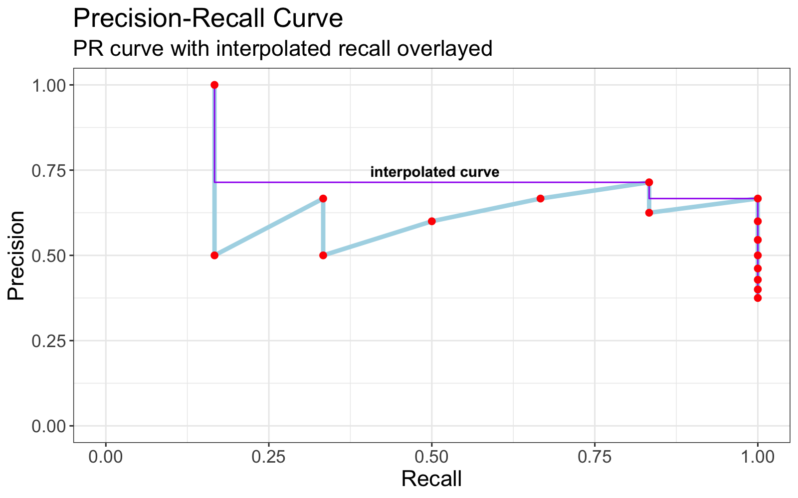
Some authors use interpolated precision whereby the Precision-Recall curve is transformed such that the precision at recall \(r\) is taken to be the \(max(precision)\) at all \(recall \ge r\).

Precision at k (P@k)¶

Precision at k measures What percent of the top k ranked predictions are true instances? This is useful in settings like information retrieval where one only cares about the top k ranked documents returned by a search query.

Example¶

Suppose we build a system that predicts which movies are relevant to a particular search query (e.g. "dog movies"). Our database contains 12 movies which receive the following prediction scores and prediction classes.

# pred_class = True implies we *predict* the movie is relevant.
# truth = True implies the movie *is* relevant.

| k  | pred_score | pred_class | truth |
|:--:|:----------:|:----------:|:-----:|
| 1  |    0.94    |    True    | False |
| 2  |    0.91    |    True    | False |
| 3  |    0.90    |    True    | True  |
| 4  |    0.66    |    True    | True  |
| 5  |    0.63    |    True    | True  |
| 6  |    0.57    |    True    | True  |
| 7  |    0.37    |   False    | False |
| 8  |    0.27    |   False    | True  |
| 9  |    0.21    |   False    | True  |
| 10 |    0.20    |   False    | True  |
| 11 |    0.18    |   False    | False |
| 12 |    0.06    |   False    | False |

Filter the the top 5 instances by pred_score.

| k  | pred_score | pred_class | truth |
|:--:|:----------:|:----------:|:-----:|
| 1  |    0.94    |    True    | False |
| 2  |    0.91    |    True    | False |
| 3  |    0.90    |    True    | True  |
| 4  |    0.66    |    True    | True  |
| 5  |    0.63    |    True    | True  |

Count the true instances (i.e. relevant movies).

| k  | pred_score | pred_class | truth |
|:--:|:----------:|:----------:|:-----:|
| 1  |    0.94    |    True    | False |
| 2  |    0.91    |    True    | False |
| 3  |    0.90    |    True    | True  | <- True instance
| 4  |    0.66    |    True    | True  | <- True instance
| 5  |    0.63    |    True    | True  | <- True instance

Divide by k

\[ \text{Precision @ 5} =\frac{3}{5} = 0.6 \]

Edge Cases¶

What if there are fewer than \(k\) True instances (relevant documents)?

This scenario presents a drawback to \(\text{Precision @ k}\). If there are a total of \(n\) True instances (relevant documents) where \(n < k\), the model will have at most \(\text{Precision @ k} = \frac{n}{k} < 1\).
What if there are fewer than \(k\) True predictions (retrieved documents)?

If a model returns \(m < k\) True predictions (retrieved documents), one possible implementation is to treat the next \(k - m\) predictions as False Positive predictions (irrelevant documents).

Average Precision at k (AP@k)¶

Average Precision at k represents Average Precision amongst the top k classification thresholds (cutoffs). It can also be described as area below the Precision Recall curve, restricted to the top k thresholds, and normalized by the lesser of k and the total number of true instances (relevant documents).

Ambiguity

The term Average Precision at k usually implies (Average Precision) @ k, not Average (Precision @ K). These are distinctly different!

Formula¶

\[ \operatorname {AP@k} ={\frac {\sum _{i=1}^{k}P(i)\times \operatorname {rel} (i)}{\min(k, \text{total true instances})}} \]

where \(\operatorname {rel} (i)\) is an indicator function equaling 1 if the item at rank \(i\) is a true instance, 0 otherwise.

Example¶

Given the following predictions and truths, calculate \(\operatorname {AP@3}\).

| k  | pred_score | truth |
|:--:|:----------:|:-----:|
| 1  |   0.840    | TRUE  |
| 2  |   -0.085   | TRUE  |
| 3  |   -0.264   | FALSE |
| 4  |   -0.463   | TRUE  |
| 5  |   -0.551   | TRUE  |
| 6  |   -0.579   | FALSE |
| 7  |   -0.708   | FALSE |
| 8  |   -1.108   | FALSE |
| 9  |   -1.170   | FALSE |
| 10 |   -1.593   | FALSE |

Filter the top k=3 entries by highest prediction score.

| k  | pred_score | truth |
|:--:|:----------:|:-----:|
| 1  |   0.840    | TRUE  |
| 2  |   -0.085   | TRUE  |
| 3  |   -0.264   | FALSE |

Calculate precision at each of these cutoffs.

| k | pred_score | truth | precision |
|:-:|:----------:|:-----:|:---------:|
| 1 |   0.840    | TRUE  |   1.00    |
| 2 |   -0.085   | TRUE  |   1.00    |
| 3 |   -0.264   | FALSE |   0.67    |

Sum the precisions of relevant documents (true instances)

| k | pred_score | truth | precision |
|:-:|:----------:|:-----:|:---------:|
| 1 |   0.840    | TRUE  |   1.00    | <- include
| 2 |   -0.085   | TRUE  |   1.00    | <- include
| 3 |   -0.264   | FALSE |   0.67    |

\[ \sum _{i=1}^{3}P(i)\times \operatorname {rel} (i) = 1.00 + 1.00 = 2.00 \]

Normalize by the lesser of \(k\) and the total number of relevant documents (true instances)

In this example, the total number of true instances is 4.

\[ \operatorname {AP@k} ={\frac {\sum _{i=1}^{3}P(i)\times \operatorname {rel} (i)}{\min(k, \text{total true instances})}} = \frac{2.00}{\min(3, 4)} = \frac{2}{3} = 0.67 \]

Intuition
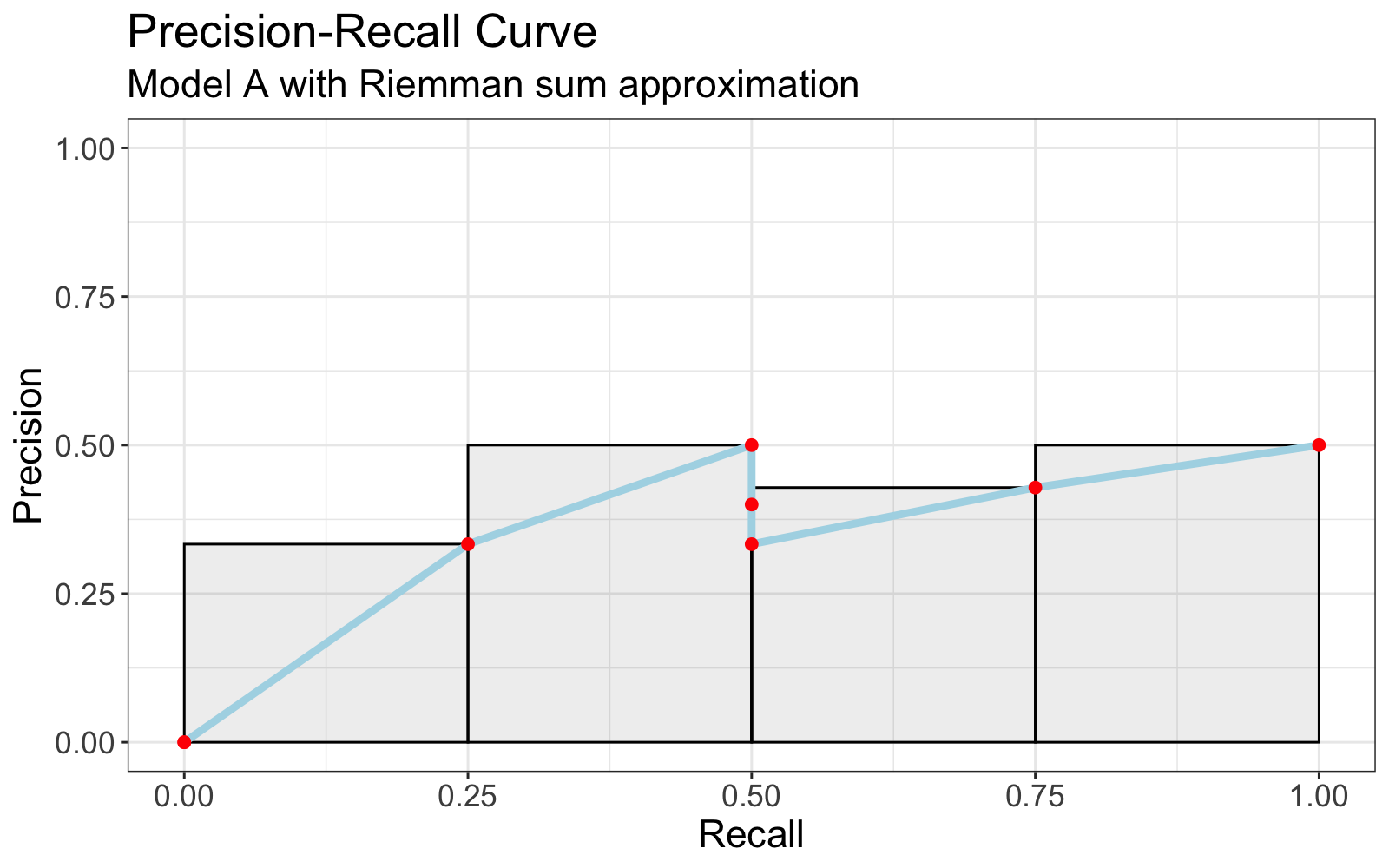
Observe the Precision-Recall curve for this example.

Average precision measures the area under the curve, which we can approximate with a Reimann sum.

Average Precision at 3 corresponds to area beneath the precision recall curve restricted to the first three cutoffs in the ordered predictions. In other words, the area beneath the curve to the left of the third point.

However the rectangle widths are rescaled to have width \(\frac{1}{3}\) so that the maximum achievable area beneath the curve in this range is 1. This is the purpose of the denominator, \(\min(k, \text{total true instances})\) in the formula for \(\operatorname {AP@k}\).

Mean Average Precision (MAP)¶

Mean Average Precision calculates Average Precision for Q queries and averages their results.

Formula¶

\[ \operatorname{MAP} = \frac{\sum_{q=1}^Q \operatorname{AP(q)}}{Q} \! \]

Mean Average Precision at k (MAP@k)¶

Mean Average Precision at k calculates Average Precision at k for Q queries and averages their results.

Formula¶

\[ \operatorname{MAP@k} = \frac{\sum_{q=1}^Q \operatorname{AP@k(q)}}{Q} \! \]