Beginner
Why use NumPy Arrays?
NumPy arrays are a lot like Python lists, but
- arrays are faster than lists (for accessing data)
- lists can store mixed types (e.g. ints and floats). The data in an array must be of the same type (e.g. ints or floats but not both).
Because arrays contain a homogeneous data type, you can do things like sum() an array of floats without worry
that one of those elements might be a string.
Basic Array Operations
Make a 1-d array
You can make a 1-d array from a list.
arr = np.array([10, 20, 30, 40, 50])
Print the array
print(arr)
# [10 20 30 40 50]
Check its dimensionality
print(arr.ndim)
# 1
Check its shape
print(arr.shape)
# (5,)
Check how many elements are in the array
len(arr)
# 5
Make a 2-d array
You can make a 2-d array from a list of lists.
arr_2d = np.array([
    [10, 20, 30, 40, 50],
    [100, 200, 300, 400, 500]
])

print(arr_2d)
# [[ 10  20  30  40  50]
#  [100 200 300 400 500]]
Check its dimensionality
print(arr_2d.ndim)
# 2
Check its shape
print(arr_2d.shape)
# (2, 5)
Check its length
print(len(arr_2d))
# 2
Tip
You might be surprised to see arr_2d has length 2, not 10. That's because arr_2d can be interpreted as an
array that contains 2 arrays inside it. If you want to get the total number of nested elements in the array, you
can use the array size attribute.
Check how many elements are in the array
print(arr_2d.size)
# 10
Check the object's type
type(arr_2d) # (1)!
# <class 'numpy.ndarray'>
- Nothing special here;
type()is a built-in Python function for identifying the type of any Python object.
Check what type of data the array contains
arr_2d.dtype
# int64
Rules For Every NumPy Array
There are two basic rules for every numpy array..
- Every element in the array must be of the same type and size.
- If an array's elements are also arrays, those inner arrays must have the same type and number of elements as each other. In other words, multidimensional arrays must be rectangular, not jagged.
Good:
np.array([1, 2, 3])
Bad:
np.array([1, 'hello', 3])
#  array(['1', 'hello', '3'], dtype='<U21')
Attention
If you try to make an array from a list that contains a mix of integers and strings, numpy doesn't error. But, it casts the integers to strings in order to satisfy the property that every element is the same type.
Bad:
np.array([
    [1, 2, 3, 4],
    [5, 6]
])
# array([list([1, 2, 3, 4]), list([5, 6])], dtype=object)
Attention
If you try to make an array from jagged lists like this, numpy doesn't error but it creates an array of objects. This means the array is essentially a Python list and lacks the performance benefits of using an array.
Creating NumPy Arrays
How to make a 1-d array from a list
np.array(['a', 'b', 'c'])
How to make a 2-d array from a list of lists
np.array([
    ['a', 'b'],
    ['c', 'd'],
    ['e', 'f']
])
How to make a 3-d array from a list of lists of lists
np.array([
    [
        ['a', 'b'],
        ['c', 'd'],
        ['e', 'f']
    ],
    [
        ['g', 'h'],
        ['i', 'j'],
        ['k', 'l']
    ]
])
Info
You can make follow this pattern to create higher dimensional arrays.
How to make an array of zeros
A quick google search will lead you to the numpy documentation for numpy.zeros.
Make a (3,) array of 0s
np.zeros(shape=3)
# array([0., 0., 0.])
Make a (3,5) array of 0s
np.zeros(shape=(3,5))
# array([[0., 0., 0., 0., 0.],
#        [0., 0., 0., 0., 0.],
#        [0., 0., 0., 0., 0.]])
How to make an array filled with any value
See numpy.full.
np.full(shape = (3,5), fill_value = 'cat')
# array([['cat', 'cat', 'cat', 'cat', 'cat'],
#        ['cat', 'cat', 'cat', 'cat', 'cat'],
#        ['cat', 'cat', 'cat', 'cat', 'cat']], dtype='<U3')
How to make a sequence array 1, 2, ... N
np.arange(start=1, stop=5, step=1)
# array([1, 2, 3, 4])
Note
Note that start is inclusive while stop is exclusive.
Alternatively:
np.arange(4)
# array([0, 1, 2, 3])
Indexing 1-D Arrays
Start by making a 1d array called foo with five elements.
foo = np.array([10, 20, 30, 40, 50])

print(foo)
# [10 20 30 40 50]
Access the ith element of an array
We can access the ith element just like a python list using square bracket notation where the first element starts at index zero.
print(foo) # (1)!
# [10 20 30 40 50]

foo[0]  # 10, 1st element
foo[1]  # 20, 2nd element
-
foo = np.array([10, 20, 30, 40, 50])
Modify the ith element
Set the 2nd element to 99
print(foo) # (1)!
# [10 20 30 40 50]

foo[1] = 99

print(foo)
# [10 99 30 40 50]
-
foo = np.array([10, 20, 30, 40, 50])
Access the last element
print(foo)
# [10 20 30 40 50]

print(foo[4])
# 50
print(foo)
# [10 20 30 40 50]

print(foo[len(foo) - 1])
# 50
print(foo)
# [10 20 30 40 50]

print(foo[-1])
# 50
Negative Indexing
Just like python lists, we can use negative indexing..
print(foo)
# [10 20 30 40 50]

print(foo[-1])  # 50, last element
print(foo[-2])  # 40, 2nd-to-last element
print(foo[-3])  # 30, 3rd-to-last element
Out of bounds error
If we try to access an element outside the bounds of the array, we’ll get an “out of bounds” error.
print(foo)
# [10 20 30 40 50]

print(foo[999])
# IndexError: (1)
- IndexError: index 999 is out of bounds for axis 0 with size 5
Accessing multiple elements
We can access multiple elements using a list or numpy array of indices.
Example
print(foo)
# [10 20 30 40 50]

print(foo[[0, 1, 4]])
# [ 10, 20,  50]
Indices can be repeated..
print(foo)
# [10 20 30 40 50]

print(foo[[0, 1, 0]])
# [ 10, 20,  10]
Indices can be another numpy array
print(foo)
# [10 20 30 40 50]

print(foo[np.zeros(shape=3, dtype='int64')]) # (1)!
# array([10, 10, 10])
- Note the use of
dtype='int64'. By default,np.zerosreturns floats, but array indices need to be integers.
Array Slicing
We can use slicing just like python lists. The signature is essentially
foo[ start index : end index : step size ]
Note
Note that start index is inclusive while end index is exclusive.
Get every element from the beginning of the array to index 2 exclusive
print(foo)
# [10 20 30 40 50]

print(foo[:2])
# [ 10, 20]
Get every element from index 2 inclusive to the end of the array
print(foo)
# [10 20 30 40 50]

print(foo[2:])
# [30, 40, 50]
Get every other element from the beginning of the array to the end
print(foo)
# [10 20 30 40 50]

print(foo[::2])
# [10, 30, 50]
Modifying multiple elements
If you want to modify multiple elements of a 1-d array, you can use a list of indices and a list of assignment values. The list of assignment values should be the same length as the list of indices.
print(foo)
# [10 20 30 40 50]

foo[[0, 1, 4]] = [100, 200, 400]

print(foo)
# [100 200  30  40 400]
..or you can assign everything to a scalar.
print(foo)
# [10 20 30 40 50]

foo[[0, 1, 4]] = 99

print(foo)
# [99 99 30 40 99]
Indexing Multidimensional Arrays
Start by making a new (3,4) array called bar from a list of lists.
bar = np.array([
    [5, 10, 15, 20],
    [25, 30, 35, 40],
    [45, 50, 55, 60]
])
Internally, bar is just a contiguous block of memory storing some data. Since we defined bar using a list of lists,
numpy makes it a two-dimensional array, giving it two axes for indexing its values.
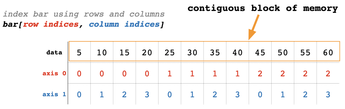
Since bar has two axes (dimensions), numpy knows to interpret the data as a rectangular array where axis 0 is the row
axis and axis 1 is the column axis. This means we can subset bar using a combination of row indices and column
indices.
Get element in the 2nd row, third column
print(bar)
# [[ 5 10 15 20]
#  [25 30 35 40]
#  [45 50 55 60]]

print(bar[1, 2])
# 35
Get first row as a 1-d array
print(bar)
# [[ 5 10 15 20]
#  [25 30 35 40]
#  [45 50 55 60]]

print(bar[0])
# [ 5 10 15 20]
Get first row as a 2-d array
print(bar)
# [[ 5 10 15 20]
#  [25 30 35 40]
#  [45 50 55 60]]

print(bar[0, None])
# [[ 5 10 15 20]]
We’ll learn more about the None keyword later. Alternatively, you can use slicing for the row index.
print(bar)
# [[ 5 10 15 20]
#  [25 30 35 40]
#  [45 50 55 60]]

print(bar[:1])
# [[ 5 10 15 20]]
Get rows 2 & 3 with the 2nd-to-last and last columns
print(bar)
# [[ 5 10 15 20]
#  [25 30 35 40]
#  [45 50 55 60]]

print(bar[1:3, [-2, -1]])
# [[35 40]
#  [55 60]]
Modifying multiple elements
Replace the top left element of bar with -1
print(bar)
# [[ 5 10 15 20]
#  [25 30 35 40]
#  [45 50 55 60]]

bar[0, 0] = -1
print(bar)
# [[-1 10 15 20]
#  [25 30 35 40]
#  [45 50 55 60]]
Replace the second row with the third row
print(bar)
# [[ 5 10 15 20]
#  [25 30 35 40]
#  [45 50 55 60]]

bar[1] = bar[2]
print(bar)
# [[ 5 10 15 20]
#  [45 50 55 60]
#  [45 50 55 60]]
Insert zeros on diagonal
print(bar)
# [[ 5 10 15 20]
#  [25 30 35 40]
#  [45 50 55 60]]

bar[[0, 1, 2], [0, 1, 2]] = [0, 0, 0]
print(bar)
# [[ 0 10 15 20]
#  [25  0 35 40]
#  [45 50  0 60]]
Notice here that the ith row index and the ith column index combine to select a specific array element. For
example, row index 1 combines with column index 1 to select element bar[[1,1]] of bar.
Interpreting Multidimensional Arrays
It's natural to interpret a three-dimensional array as a rectangular prism like this.
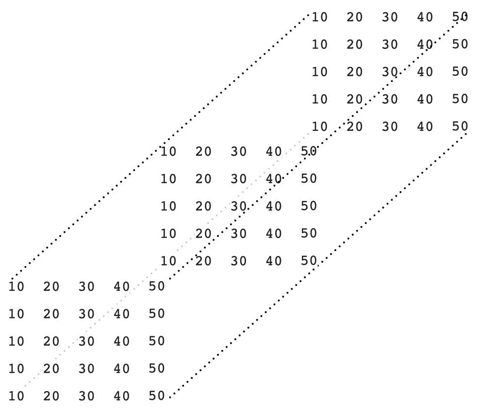
Unfortunately, this spacial model breaks down when you go above three dimensions. A better mental model is to interpret a 1-dimensional array as a row of numbers
a two-dimensional array as a matrix (rows and columns)
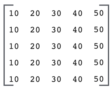
a three-dimensional array as a row of matrices
a four-dimensional array as a matrix of matrices
and so on. Now if you have a three-dimensional array like this
zoo = np.array([
    [
        [10,20],
        [30,40],
        [50,60],
    ],
    [
        [11,12],
        [13,14],
        [15,16],
    ]
])

print(zoo)
# [[[10 20]
#   [30 40]
#   [50 60]]
#  [[11 12]
#   [13 14]
#   [15 16]]]
and you make an assignment like zoo[0,:,1] = 5, you can interpret the assignment as
set the 1st matrix, every row, 2nd column equal to 5
zoo[0,:,1] = 5

print(zoo)
# [[[10  5]
#   [30  5]
#   [50  5]]
#  [[11 12]
#   [13 14]
#   [15 16]]]
Attention
We've glossed over some gritty details and complex scenarios regarding array indexing which we'll cover later.
Basic Math on Arrays
Start by defining a pair of 2x2 arrays, foo and bar.
foo = np.array([[4,3], [1,0]])
bar = np.array([[1,2], [3,4]])

print(foo)
# [[4 3]
#  [1 0]]

print(bar)
# [[1 2]
#  [3 4]]
Addition
See what happens when we add foo + bar
foo + bar
# array([[5, 5],
#        [4, 4]])
The values of foo and bar get added element-wise. This pattern of element-wise addition holds true for every math operation between identically sized arrays.
Subtraction
foo - bar
# array([[ 3,  1],
#        [-2, -4]])
Multiplication
foo * bar
# array([[4, 6],
#        [3, 0]])
Division
foo / bar
# array([[4.        , 1.5       ],
#        [0.33333333, 0.        ]])
Matrix Multiplication
Use the @ operator to do matrix multiplication between numpy arrays.
foo @ bar
# array([[13, 20],
#        [ 1,  2]])
Broadcasting Arithmetic
If you do foo + 5, numpy adds 5 to each element of foo.
foo + 5
# array([[9, 8],
#        [6, 5]])
The same goes for subtraction multiplication, division, and all other binary arithmetic operations. This behavior is known as broadcasting. We'll discuss broadcasting in detail later.