DataFrame

What's a DataFrame?¶

A pandas DataFrame is a table of data. More specifically, it's a collection of 1-D arrays of the same length, that share a row index and a column index.

DataFrame is similar to a 2-D NumPy array, but with DataFrame, each column can store a different type of data. For example, here's a DataFrame with a column of ints, a column of strings, and a column of Dates.

df = pd.DataFrame({
    'Messages': [43,0,7,32,2,5], 
    'Sender': ['Mom', 'Dad', 'Girlfriend', 'Mom', 'Dad', 'Girlfriend'],
    'Date': pd.to_datetime(['2022-01-22', '2022-01-22', '2022-01-22', '2022-01-23', '2022-01-23', '2022-01-23'])
})

print(df)
#    Messages      Sender       Date
# 0        43         Mom 2022-01-22
# 1         0         Dad 2022-01-22
# 2         7  Girlfriend 2022-01-22
# 3        32         Mom 2022-01-23
# 4         2         Dad 2022-01-23
# 5         5  Girlfriend 2022-01-23

DataFrame Creation¶

DataFrame From Dictionary¶

Perhaps the easiest way to make a DataFrame from scratch is to use the DataFrame() constructor, passing in a dictionary of column_name:columns_values pairs.

Example:

df = pd.DataFrame({
    'name': ['Bob', 'Sue', 'Mary'], 
    'age': [39, 57, 28]
})

print(df)
#    name  age
# 0   Bob   39
# 1   Sue   57
# 2  Mary   28

DataFrame From List Of Lists¶

You can build a DataFrame from a list of lists where each inner list represents a row of the DataFrame.

df = pd.DataFrame([
    ['Bob', 39],
    ['Sue', 57],
    ['Mary', 28]
], columns=['name', 'age'])

print(df)
#    name  age
# 0   Bob   39
# 1   Sue   57
# 2  Mary   28

DataFrame Inspection¶

DataFrame has a number of handy tools for inspection..

df = pd.DataFrame({
    'name': ['Bob', 'Sue', 'Mary'], 
    'age': [39, 57, 28]
})

print(df)
#    name  age
# 0   Bob   39
# 1   Sue   57
# 2  Mary   28

`DataFrame.info()`¶

reports information about the DataFrame's structure.

df.info()

# <class 'pandas.core.frame.DataFrame'>
# RangeIndex: 3 entries, 0 to 2
# Data columns (total 2 columns):
#  #   Column  Non-Null Count  Dtype 
# ---  ------  --------------  ----- 
#  0   name    3 non-null      object
#  1   age     3 non-null      int64 
# dtypes: int64(1), object(1)
# memory usage: 176.0+ bytes

`DataFrame.shape`¶

returns a tuple with the number of rows and columns in the DataFrame.

df.shape
# (3, 2)

`DataFrame.axes`¶

returns a list with the DataFrame's row index and column index.

df.axes
# [RangeIndex(start=0, stop=3, step=1), Index(['name', 'age'], dtype='object')]

`DataFrame.size`¶

returns the total number of elements in the DataFrame.

df.size
# 6

To And From CSV¶

`DataFrame.to_csv()`¶

To write a DataFrame to CSV, use the DataFrame.to_csv() method.

df = pd.DataFrame({
    'id': [0,3,9],
    'b': [12.5, 42.1, 905.3],
    'c': pd.Series(['cat', 'dog', 'hippo'], dtype="string")
})  # (1)!

print(df)
#    id      b      c
# 0   0   12.5    cat
# 1   3   42.1    dog
# 2   9  905.3  hippo

# Save df as a CSV file in the current working directory
df.to_csv('pets.csv')

You might be thinking, "Hey! A hippo isn't a pet!" Prepare to stand corrected.

By default, to_csv() writes the DataFrame to your current working directory. You can check your current working directory using the getcwd() function from os.

import os
os.getcwd()  # /Users/scooby/PracticeProbs/Pandas

Alternatively, you can write the DataFrame to a specific file path using the path_or_buf parameter.

df.to_csv(path_or_buf='/some/special/path/pets.csv')

Row Index Column¶

By default, to_csv() includes the row index in the output. For example, df.to_csv('pets.csv') above would generate a CSV file that looks like this.

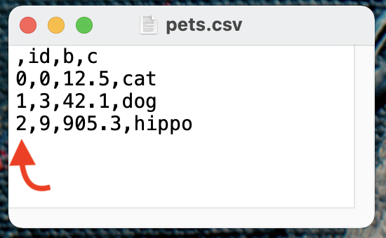
Notice the nameless column at the front. If you want to exclude the row index, set index=False within to_csv().

# Write df to CSV excluding the row index
df.to_csv('pets.csv', index=False)

`pandas.read_csv()`¶

You can create a DataFrame from a CSV file using the read_csv() function, passing in the name of the file.

# Load 'pets.csv' into a DataFrame called pets
df = pd.read_csv('pets.csv')  # (1)!

print(df)
#    id      b      c
# 0   0   12.5    cat
# 1   3   42.1    dog
# 2   9  905.3  hippo

Here, pets.csv is expected to live in your current working directory. Alternatively, you can provide a relative path to the file like data/pets.csv or an absolute path like /Users/scooby/pets.csv.

In the real world, reading CSV files doesn't always go smoothly. Sometimes you'll have to steer read_csv() in the right direction using some parameters like

sep to specify a value separator if your file is something other than comma delimited
header to tell pandas if your file contains column names
index_col to indicate which column if any should be used as the row index
usecols to tell pandas "only read a certain subset of columns"

Basic Indexing¶

Indexing a DataFrame is very similar to indexing a Series..

df = pd.DataFrame({
    'shrimp': [10, 20, 30, 40, 50, 60],
    'crab': [5, 10, 15, 20, 25, 30],
    'red fish': [2, 3, 5, 7, 11, 13]
})

print(df)
#    shrimp  crab  red fish
# 0      10     5         2
# 1      20    10         3
# 2      30    15         5
# 3      40    20         7
# 4      50    25        11
# 5      60    30        13

Indexing Columns¶

Access column as a Series¶

To access a DataFrame column as a Series, reference its name using square bracket notation or dot notation.

square bracket notationdot notation

df['shrimp']
# 0    10
# 1    20
# 2    30
# 3    40
# 4    50
# 5    60
# Name: shrimp, dtype: int64

df.shrimp

# 0    10
# 1    20
# 2    30
# 3    40
# 4    50
# 5    60
# Name: shrimp, dtype: int64

Dot notation only works if the column name has alphanumeric characters only. If the name has a space, tilde, etc. you must use square bracket notation.

If you'd like to get the result as a one-column DataFrame instead of a Series, use square bracket indexing with the column name wrapped inside a list.

df[['shrimp']]
#    shrimp
# 0      10
# 1      20
# 2      30
# 3      40
# 4      50
# 5      60

Access columns by name¶

You can access one or more columns using square bracket notation, passing in a list of column names.

df[['shrimp', 'crab']]
#    shrimp  crab
# 0      10     5
# 1      20    10
# 2      30    15
# 3      40    20
# 4      50    25
# 5      60    30

The result is a DataFrame whose data is a copy of the original DataFrame.

Access columns by position¶

You can also use DataFrame.iloc to select columns by position. For example, df.iloc[:, [0, 1]] returns every row of the DataFrame, but only columns 0 and 1.

df.iloc[:, [0, 1]]
#    shrimp  crab
# 0      10     5
# 1      20    10
# 2      30    15
# 3      40    20
# 4      50    25
# 5      60    30

df.iloc[[0, 2], [1, 2]] returns rows 0 and 2 with columns 1 and 2.

df.iloc[[0, 2], [1, 2]]
#    crab  red fish
# 0     5         2
# 2    15         5

Indexing Rows¶

Access rows by position¶

If you want to pick out certain rows of a DataFrame by their position, you can use DataFrame.iloc[], very similar to Series.iloc[].

For example, to get the 1st, 3rd, and 5th rows of df, you could do

df.iloc[[0, 2, 4]]
#    shrimp  crab  red fish
# 0      10     5         2
# 2      30    15         5
# 4      50    25        11

Alternatively, you can use slicing.

df.iloc[0:5:2]
#    shrimp  crab  red fish
# 0      10     5         2
# 2      30    15         5
# 4      50    25        11

If you select an individual row with iloc like this

df.iloc[1]
# shrimp      20
# crab        10
# red fish     3
# Name: 1, dtype: int64

the result is a Series, not a DataFrame.

To fetch an individual row of a DataFrame as a DataFrame, you pass in a list of indices.

df.iloc[[1]]
#    shrimp  crab  red fish
# 1      20    10         3

Access rows by index label¶

You can use DataFrame.loc[] to access rows of a DataFrame by index label. For example, given a DataFrame whose row index is the letters 'a' through 'f',

df = pd.DataFrame({
    'shrimp': [10, 20, 30, 40, 50, 60],
    'crab': [5, 10, 15, 20, 25, 30],
    'red fish': [2, 3, 5, 7, 11, 13],
}, index=['a','b','c','d','e','f'])

print(df)
#    shrimp  crab  red fish
# a      10     5         2
# b      20    10         3
# c      30    15         5
# d      40    20         7
# e      50    25        11
# f      60    30        13

we can select the rows with index labels b and e using df.loc[['b', 'e']].

df.loc[['b', 'e']]
#    shrimp  crab  red fish
# b      20    10         3
# e      50    25        11

We can combine row and column indexing to select rows a, c, and f with columns crab and shrimp.

df.loc[['a', 'c', 'f'], ['crab', 'shrimp']]
#    crab  shrimp
# a     5      10
# c    15      30
# f    30      60

And we can even use slicing to pick out every row between b and e for column crab.

df.loc['b':'e', ['crab']]
#    crab
# b    10
# c    15
# d    20
# e    25

Boolean Indexing¶

You can use boolean indexing to select rows of a DataFrame, just as you can with Series.

df = pd.DataFrame({
    'shrimp': [10, 20, 30, 40, 50, 60],
    'crab': [5, 10, 15, 20, 25, 30],
    'red fish': [2, 3, 5, 7, 11, 13],
}, index=['a','b','c','d','e','f'])

print(df)
#    shrimp  crab  red fish
# a      10     5         2
# b      20    10         3
# c      30    15         5
# d      40    20         7
# e      50    25        11
# f      60    30        13

To get the rows of df where shrimp is less than 40, start by building a boolean Series like this.

mask = df.shrimp < 40

print(mask)
# a     True
# b     True
# c     True
# d    False
# e    False
# f    False
# Name: shrimp, dtype: bool

Notice it has the same index as df; therefore we can pass it into df.loc[] to select rows where shrimp is less than 40.

df.loc[mask]
#    shrimp  crab  red fish
# a      10     5         2
# b      20    10         3
# c      30    15         5

More commonly you'll see this as a one-liner.

df.loc[df.shrimp < 40]
#    shrimp  crab  red fish
# a      10     5         2
# b      20    10         3
# c      30    15         5

Just like Series, you can combine logical conditions to create more intricate filters.

# select rows where shrimp is less than 50 and 
# crab is not divisible by 10

df.loc[(df.shrimp < 50) & ~(df.crab % 10 == 0)]
#    shrimp  crab  red fish
# a      10     5         2
# c      30    15         5

Access rows by position, columns by name¶

If you wanted to select the first three rows of df with the columns shrimp and red fish you might try

df.loc[:3, ['shrimp', 'red fish']]

or

df.iloc[:3, ['shrimp', 'red fish']]

but both of these techniques fail.

df.loc expects label indexers, so the positional indexer :3 causes an error.
df.iloc expects positional indexers, so the label indexer ['shrimp', 'red fish'] causes an error.

One solution is to convert the column names 'shrimp', and 'red fish' to their corresponding positional indices 0 and 2, and then use iloc as usual.

df.iloc[:3, [0, 2]]
#    shrimp  red fish
# a      10         2
# b      20         3
# c      30         5

To make this dynamic, we can replace [0, 2] with
[df.columns.get_loc(c) for c in ['shrimp', 'red fish']].

df.iloc[:3, [df.columns.get_loc(c) for c in ['shrimp', 'red fish']]]  # (1)!
#    shrimp  red fish
# a      10         2
# b      20         3
# c      30         5

df.columns.get_loc() returns the positional index of a column given its name.

Note that df.columns returns the column index of the DataFrame.

df.columns
# Index(['shrimp', 'crab', 'red fish'], dtype='object')

Basic Operations¶

Inserting columns¶

You can insert a new column 'c' into an existing DataFrame df via df['c'] = x where x is either a list, Series, NumPy array, or a scalar.

df = pd.DataFrame({
    'a': [2, 3, 11, 13],
    'b': ['fox', 'rabbit', 'hound', 'rabbit']
})

print(df)
#     a       b
# 0   2     fox
# 1   3  rabbit
# 2  11   hound
# 3  13  rabbit

# insert a new column called 'c'
df['c'] = [1, 0, 1, 2]

print(df)
#     a       b  c
# 0   2     fox  1
# 1   3  rabbit  0
# 2  11   hound  1
# 3  13  rabbit  2

You can't use dot notation to create a new column. E.g. you can't do df.d = 1

You can also combine columns to create a new column. For example,

df['d'] = df.a + df.c

print(df)
#     a       b  c   d
# 0   2     fox  1   3
# 1   3  rabbit  0   3
# 2  11   hound  1  12
# 3  13  rabbit  2  15

Updating values¶

You can create or update column values using boolean indexing. For example, given the following DataFrame,

df = pd.DataFrame({
    'a': [2, 3, 11, 13],
    'b': ['fox', 'rabbit', 'hound', 'rabbit'],
})

print(df)
#     a       b
# 0   2     fox
# 1   3  rabbit
# 2  11   hound
# 3  13  rabbit

we can update a to equal 0 where b is 'rabbit' as follows

df.loc[df.b == 'rabbit', 'a'] = 0

print(df)
#     a       b
# 0   2     fox
# 1   0  rabbit
# 2  11   hound
# 3   0  rabbit

Removing columns¶

To remove columns from a DataFrame, use DataFrame.drop() passing in a list of column names to the columns argument.

df = pd.DataFrame({
    'a': [2, 3, 11, 13],
    'b': ['fox', 'rabbit', 'hound', 'rabbit'],
    'c': [9, 4, 12, 12]
})
df.drop(columns=['a', 'c'])  # (1)!
#         b
# 0     fox
# 1  rabbit
# 2   hound
# 3  rabbit

df.drop(columns=['a', 'c']) creates a new DataFrame that's a copy of df without columns a and c. If you want to modify df instead of copying it, use df.drop(columns=['a', 'c'], inplace=True).

Changing column names¶

To change a DataFrame's column names, use the DataFrame.rename() method passing in a dictionary of old_name:new_name pairs.

For example, here we change the column name 'age' to 'years'.

df = pd.DataFrame({
    'name': ['Bob', 'Sue', 'Mary'], 
    'age': [39, 57, 28]
})
print(df)
#    name  age
# 0   Bob   39
# 1   Sue   57
# 2  Mary   28

df.rename(columns={'age':'years'}, inplace=True)  # (1)!
print(df)
#    name  years
# 0   Bob     39
# 1   Sue     57
# 2  Mary     28

Here we modify df "in place". Without inplace=True we'd get back a copy of df with the new column names.

`DataFrame.apply()`¶

DataFrame's apply() method lets you apply a function to each row or column in a DataFrame. apply() has two primary arguments:

func: tells apply() what function to apply
axis: tells apply() whether to apply the function to each column (axis=0) or each row (axis=1)

For example, given the following DataFrame

df = pd.DataFrame({
    'A': [5.2, 1.7, 9.4],
    'B': [3.9, 4.0, 7.8]
})

print(df)
#      A    B
# 0  5.2  3.9
# 1  1.7  4.0
# 2  9.4  7.8

calling df.apply(func=np.sum, axis=0) sums the data in each column.

df.apply(func=np.sum, axis=0)
# A    16.3
# B    15.7
# dtype: float64

Notice the result is a 2-element Series whose index labels are the column names of df.

The same operation with axis=1 generates a 3-element Series with the sum of each row.

df.apply(func=np.sum, axis=1)
# 0     9.1
# 1     5.7
# 2    17.2
# dtype: float64

apply() with function arguments¶

Now suppose we have a DataFrame called kids with mixed column types..

kids = pd.DataFrame({
    'name': pd.Series(['alice', 'mary', 'jimmy', 'johnny', 'susan'], dtype="string"),
    'age': [9, 13, 11, 15, 8],
    'with_adult': [True, False, False, True, True]
})

print(kids)
#      name  age  with_adult
# 0   alice    9        True
# 1    mary   13       False
# 2   jimmy   11       False
# 3  johnny   15        True
# 4   susan    8        True

Our goal is to determine whether each child should be allowed in a haunted house. To be allowed inside,

you must be at least 12 years old or
you must have adult supervision

apply() works great for tasks like this.

We start by making a function called is_allowed() that inputs a number, age, and a boolean, with_adult, and returns a boolean indicating whether that kid is allowed to enter the haunted house.

def is_allowed(age, with_adult):
    return age >= 12 or with_adult

To apply this function to each row, you may be inclined to try

kids.apply(is_allowed, axis=1)

but this fails because pandas doesn't know which columns to use for the age and with_adult parameters of the is_allowed() function.

It's important to understand that the input to the function is a Series representation of the "current row". For example, the Series representation of the first row of kids looks like this

x = kids.iloc[0]

print(x)
# name          alice
# age               9
# with_adult     True
# Name: 0, dtype: object

Passing this result into the is_allowed() function fails for numerous reasons.

is_allowed(x)  # error (1)

TypeError: is_allowed() missing 1 required positional argument: 'with_adult'

To overcome this, we create a wrapper function for is_allowed() using lambda as follows.

kids.apply(lambda x: is_allowed(x.loc['age'], x.loc['with_adult']), axis=1)
# 0     True
# 1     True
# 2    False
# 3     True
# 4     True
# dtype: bool

Tacking that onto our kids DataFrame, we can see exactly who's allowed in the haunted house.

kids['allowed'] = kids.apply(
    lambda x: is_allowed(x.loc['age'], x.loc['with_adult']), 
    axis=1
)

print(kids)
#      name  age  with_adult  allowed
# 0   alice    9        True     True
# 1    mary   13       False     True
# 2   jimmy   11       False    False (1)
# 3  johnny   15        True     True
# 4   susan    8        True     True

Beat it, Jimmy!

Merging DataFrames¶

The workhorse function to merge DataFrames together is merge().

To motivate its use, suppose we have the following two tables of data:

pets: one row per pet. The index represents each pet_id
visits one row per visit. The index represents each visit_id

pets = pd.DataFrame(
    data={
        'name': ['Mr. Snuggles', 'Honey Chew Chew', 'Professor', 'Chairman Meow', 'Neighbelline'],
        'type': ['cat', 'dog', 'dog', 'cat', 'horse']
    },
    index=[71, 42, 11, 98, 42]
)

visits = pd.DataFrame(
    data={
        'pet_id': [42, 31, 71, 42, 98, 42],
        'date': ['2019-03-15', '2019-03-15', '2019-04-05', '2019-04-06', '2019-04-12', '2019-04-12']
    }
)

print(pets)
#                name   type
# 71     Mr. Snuggles    cat
# 42  Honey Chew Chew    dog
# 11        Professor    dog
# 98    Chairman Meow    cat
# 42     Neighbelline  horse

print(visits)
#    pet_id        date
# 0      42  2019-03-15
# 1      31  2019-03-15
# 2      71  2019-04-05
# 3      42  2019-04-06
# 4      98  2019-04-12
# 5      42  2019-04-12

merge() has four types of joins: left, right, inner, and outer, with the default being inner. The join type determines which keys show up in the result.

Inner Join¶

The result of an inner join only includes keys that exist in both the left and right tables. (A single key can appear multiple times in the result if it appears multiple times in one of the input tables.)

Here we,

designate pets as the left table
designate visits as the right table
set the join type as inner
set left_index=True because in the left table (pets), pet ids are stored in the row index
set right_on='pet_id' because in the right table (visits), pet ids are stored in a column called pet_id

# inner join between pets and visits based on pet_id
pd.merge(
    left=pets, 
    right=visits, 
    how='inner', 
    left_index=True, 
    right_on='pet_id'
)
#               name   type  pet_id        date
# 2     Mr. Snuggles    cat      71  2019-04-05
# 0  Honey Chew Chew    dog      42  2019-03-15
# 3  Honey Chew Chew    dog      42  2019-04-06
# 5  Honey Chew Chew    dog      42  2019-04-12
# 0     Neighbelline  horse      42  2019-03-15
# 3     Neighbelline  horse      42  2019-04-06
# 5     Neighbelline  horse      42  2019-04-12
# 4    Chairman Meow    cat      98  2019-04-12

Notice:

pet_id 11 is excluded because it only exists in the pets table and pet_id 31 is excluded because it only exists in the visits table.
pet_id 42 occurs six times in result because it occurred three times in the visits table, each of which matched two occurrences in the pets table.

When your DataFrame's row index has some specific meaning (kind of like ours), it's a good practice to give it a name. Here we rename the row index of pets to pet_id.

pets.index.rename('pet_id', inplace=True)

print(pets)
#                    name   type
# pet_id                        
# 71         Mr. Snuggles    cat
# 42      Honey Chew Chew    dog
# 11            Professor    dog
# 98        Chairman Meow    cat
# 42         Neighbelline  horse

We'll also rename the row index of visits to visit_id.

visits.index.rename('visit_id', inplace=True)

print(visits)
#           pet_id        date
# visit_id                    
# 0             42  2019-03-15
# 1             31  2019-03-15
# 2             71  2019-04-05
# 3             42  2019-04-06
# 4             98  2019-04-12
# 5             42  2019-04-12

A convenient benefit to naming the pet_id index is that we can rebuild the inner join from before using on='pet_id' instead of setting left_index=True and right_on='pet_id'.

pd.merge(left=pets, right=visits, how='inner', on='pet_id')
#    pet_id             name   type        date
# 0      71     Mr. Snuggles    cat  2019-04-05
# 1      42  Honey Chew Chew    dog  2019-03-15
# 2      42  Honey Chew Chew    dog  2019-04-06
# 3      42  Honey Chew Chew    dog  2019-04-12
# 4      42     Neighbelline  horse  2019-03-15
# 5      42     Neighbelline  horse  2019-04-06
# 6      42     Neighbelline  horse  2019-04-12
# 7      98    Chairman Meow    cat  2019-04-12

When you use the on parameter like this, pandas searches both tables for a matching column name and/or row index to merge the tables with. Also notice that this result is slightly different from our previous version - specifically the resulting row index is different and the resulting column order is different. I'll touch on that a bit later.

Left Join¶

The result of a left join retains all and only the keys in the left table. Let's see it in action, again making pets the left table and visits the right table, joining on pet_id.

pd.merge(left=pets, right=visits, how='left', on='pet_id')
#    pet_id             name   type        date
# 0      71     Mr. Snuggles    cat  2019-04-05
# 1      42  Honey Chew Chew    dog  2019-03-15
# 2      42  Honey Chew Chew    dog  2019-04-06
# 3      42  Honey Chew Chew    dog  2019-04-12
# 4      11        Professor    dog         NaN
# 5      98    Chairman Meow    cat  2019-04-12
# 6      42     Neighbelline  horse  2019-03-15
# 7      42     Neighbelline  horse  2019-04-06
# 8      42     Neighbelline  horse  2019-04-12

Notice:

The result includes pet_id 11 which exists in the left table (pets) but not the right table (visits).
pet_id 42 occurs six times in the result because its three instances in the left table each matched to two instances in the right table.

Right Join¶

A right join is the same as a left join, except the right table's keys are preserved.

pd.merge(left=pets, right=visits, how='right', on='pet_id')
#    pet_id             name   type        date
# 0      42  Honey Chew Chew    dog  2019-03-15
# 1      42     Neighbelline  horse  2019-03-15
# 2      31              NaN    NaN  2019-03-15
# 3      71     Mr. Snuggles    cat  2019-04-05
# 4      42  Honey Chew Chew    dog  2019-04-06
# 5      42     Neighbelline  horse  2019-04-06
# 6      98    Chairman Meow    cat  2019-04-12
# 7      42  Honey Chew Chew    dog  2019-04-12
# 8      42     Neighbelline  horse  2019-04-12

In this case, pet_id 11 is excluded but pet_id 31 is retained in the result.

Outer Join¶

The last join type supported by merge() is an outer join which includes every key from both tables in the output.

pd.merge(left=pets, right=visits, how='outer', on='pet_id')
#    pet_id             name   type        date
# 0      71     Mr. Snuggles    cat  2019-04-05
# 1      42  Honey Chew Chew    dog  2019-03-15
# 2      42  Honey Chew Chew    dog  2019-04-06
# 3      42  Honey Chew Chew    dog  2019-04-12
# 4      42     Neighbelline  horse  2019-03-15
# 5      42     Neighbelline  horse  2019-04-06
# 6      42     Neighbelline  horse  2019-04-12
# 7      11        Professor    dog         NaN
# 8      98    Chairman Meow    cat  2019-04-12
# 9      31              NaN    NaN  2019-03-15

Anti-join¶

Unfortunately merge() doesn't support anti-join which answers the question

Which records from table A don't match any records from table B?

However, cooking up an anti-join is not terribly difficult. Observe the following two techniques (and their differences).

Anti-Join Method 1¶

Suppose we want to see which records in the pets table don't have a matching record in the visits table via pet_id. we can start by doing an outer join with the indicator=True.

outer = pd.merge(
    left=pets, 
    right=visits, 
    how='outer', 
    on='pet_id', 
    indicator=True
)

print(outer)
#    pet_id             name   type        date      _merge
# 0      71     Mr. Snuggles    cat  2019-04-05        both
# 1      42  Honey Chew Chew    dog  2019-03-15        both
# 2      42  Honey Chew Chew    dog  2019-04-06        both
# 3      42  Honey Chew Chew    dog  2019-04-12        both
# 4      42     Neighbelline  horse  2019-03-15        both
# 5      42     Neighbelline  horse  2019-04-06        both
# 6      42     Neighbelline  horse  2019-04-12        both
# 7      11        Professor    dog         NaN   left_only
# 8      98    Chairman Meow    cat  2019-04-12        both
# 9      31              NaN    NaN  2019-03-15  right_only

The result includes a column named 'merge' that indicates if the corresponding record came from the _left table, the right table, or both tables. Filtering this result where _merge == 'left_only' identifies pets that don't exist in visits. This equates to an anti-join between pets and visits on pet_id.

a_not_in_b = outer.loc[outer._merge == 'left_only']

print(a_not_in_b)
#    pet_id       name type date     _merge
# 7      11  Professor  dog  NaN  left_only

This technique is simple but memory inefficient, as the outer join creates a large intermediate table.

Anti-Join Method 2¶

The second method is a little trickier, but it's more memory efficient. The basic idea is, for each pet_id in the pets table, we check if it exists in the visits table using the isin() method. Then we negate the result and use that to subset the pets table.

So if we do pets.index.isin(visits.pet_id) we get back a boolean array indicating whether each pet_id in the pets table also exists in the visits table.

pets.index.isin(visits.pet_id)
# array([ True,  True, False,  True,  True])

Then we can negate that array and use it as a boolean index to subset the pets table.

pets.loc[~pets.index.isin(visits.pet_id)]
#              name type
# pet_id                
# 11      Professor  dog

Since the visits table includes duplicate pet_ids, we can slightly improve this by using only its unique pet_ids.

pets.loc[~pets.index.isin(visits.pet_id.unique())]
#              name type
# pet_id                
# 11      Professor  dog

Aggregation¶

DataFrame's agg() method lets you aggregate the rows of a DataFrame to calculate summary statistics.

For example, given the following DataFrame,

df = pd.DataFrame({
    'x': [3.1, 5.5, 9.2, 1.7, 1.2, 8.3, 2.6],
    'y': [1.4, np.nan, 5.0, 5.8, 9.0, np.nan, 9.2]
})

print(df)
#      x    y
# 0  3.1  1.4
# 1  5.5  NaN
# 2  9.2  5.0
# 3  1.7  5.8
# 4  1.2  9.0
# 5  8.3  NaN
# 6  2.6  9.2

we can calculate the sum of each column using df.agg('sum').

df.agg('sum')
# x    31.6
# y    30.4
# dtype: float64

Or we could pass in a function callabe, like np.sum.

df.agg(np.sum)
# x    31.6
# y    30.4
# dtype: float64

Info

Aggregation is intended to be used with a special class of functions that input a Series of values and reduces them down to a single value, or at least fewer values than the input. These include functions like sum(), mean() , min(), and max().

By contrast, transformation functions like sort(), fillna(), and round() input a Series of values and return another Series the same length as the input.

When you pass a string into df.agg() like df.agg('foofunc'), pandas

first looks for a DataFrame method called 'foofunc'. If it can't find anything, it
then checks for a numpy function called 'foofunc'. If it still can't find 'foofunc', it
then raises an error.

If you defined your own function named 'foofunc', you can use it with df.agg(), but you have to pass it in as a callable.

def foofunc(x):
    return x.iloc[1]

df.agg(foofunc)    # good
df.agg('foofunc')  # bad

The result of df.agg('sum') was a 2-element Series with the sum of each column. To return the result as a DataFrame, wrap the aggregation function inside a list.

# produces a Series
df.agg('sum')
# x    31.6
# y    30.4
# dtype: float64

# produces a DataFrame
df.agg(['sum'])
#         x     y
# sum  31.6  30.4

Using a list, we can aggregate the data using multiple functions. For example, to get the sum and mean of each column,

df.agg(['sum', 'mean'])
#               x      y
# sum   31.600000  30.40
# mean   4.514286   6.08

To calculate the sum and mean of column x, and the min and max of column y, we can use a dictionary of column:list-of-functions pairs to tell pandas exactly what functions to apply to each column.

df.agg({'x': ['sum', 'mean'], 'y': ['min', 'max']})
#               x    y
# sum   31.600000  NaN
# mean   4.514286  NaN
# min         NaN  1.4
# max         NaN  9.2

DataFrame.agg() includes an axis argument. By default, it's set to 0 which tells pandas to aggregate the DataFrame's rows. This means an operation like df.agg('min') calculates column mins.

df.agg('min')  # axis=0, by default
# x    1.2
# y    1.4
# dtype: float64

By contrast, df.agg('min', axis=1) aggregates the DataFrame's columns, calculating row mins.

df.agg('min', axis=1)
# 0    1.4
# 1    5.5
# 2    5.0
# 3    1.7
# 4    1.2
# 5    8.3
# 6    2.6
# dtype: float64

DataFrame.agg() also includes *args and **kwargs parameters which can be used to pass constants into the aggregation function(s). For example, if you define some custom function like nth_value() that returns the nth value of a Series,

def nth_value(x, n):
    return x.iloc[n]

you could aggregate df, selecting the 3rd value in each column as follows.

df.agg(nth_value, n=3)
# x    1.7
# y    5.8
# dtype: float64

For simple functions like this, you'll often see people build them on the fly using lambda.

df.agg(func=lambda x, n: x.iloc[n], n=3)
# x    1.7
# y    5.8
# dtype: float64

Group By¶

You can use groupby() to partition a DataFrame or Series into groups and subsequently aggregate or transform the data in each group.

Setup

df = pd.DataFrame({
    'A': ['foo', 'bar', 'foo', 'bar', 'bar', 'foo', 'foo'],
    'B': [False, True, False, True, True, True, True],
    'C': [2.1, 1.9, 3.6, 4.0, 1.9, 7.8, 2.8],
    'D': [50, np.nan, 30, 90, 10, np.nan, 10]
}).convert_dtypes()  # (1)!

print(df)
#      A      B    C     D
# 0  foo  False  2.1    50
# 1  bar   True  1.9  <NA>
# 2  foo  False  3.6    30
# 3  bar   True  4.0    90
# 4  bar   True  1.9    10
# 5  foo   True  7.8  <NA>
# 6  foo   True  2.8    10

convert_dtypes() is a handy way to make sure we're using pandas' modern String and Integer datatypes which allow for NaN values. Without it, A would be type 'object', and D would be type 'float64'.

Every group by operation starts with a call to the groupby() method.

groupby() exists both as a Series method and as a DataFrame method.

Perhaps the most important parameter of groupby() is the by argument, which tells pandas how to split the DataFrame (or Series) into groups. Usually, you'll specify one or more column names here. For example, df.groupby(by='A') tells pandas to partition the data based on unique values in column A.

df.groupby(by='A')
# <pandas.core.groupby.generic.DataFrameGroupBy object at 0x12756a8e0>

In this case, pandas partitions the data into two groups like this

|     |  A  |   B   |  C  |   D  |
|:---:|:---:|:-----:|:---:|:----:|
|   1 | bar | True  | 1.9 | <NA> |
|   3 | bar | True  |   4 | 90   |
|   4 | bar | True  | 1.9 | 10   |
|-----|-----|-------|-----|------|
|   0 | foo | False | 2.1 | 50   |
|   2 | foo | False | 3.6 | 30   |
|   5 | foo | True  | 7.8 | <NA> |
|   6 | foo | True  | 2.8 | 10   |

Alternatively, you could do df.groupby(by=['A', 'B']) to partition the rows based on the set of unique (A, B) pairs.

df.groupby(by=['A', 'B'])
# <pandas.core.groupby.generic.DataFrameGroupBy object at 0x127572af0>

In this case, pandas partitions the data into these three groups.

|    |  A  |   B   |  C  |   D  |   
|:--:|:---:|:-----:|:---:|:----:|
|  1 | bar | True  | 1.9 | <NA> |
|  3 | bar | True  | 4   | 90   |
|  4 | bar | True  | 1.9 | 10   |
|----|-----|-------|-----|------|
|  0 | foo | False | 2.1 |  50  |
|  2 | foo | False | 3.6 |  30  | 
|----|-----|-------|-----|------|
|  5 | foo | True  | 7.8 | <NA> |
|  6 | foo | True  | 2.8 | 10   |

The result of calling DataFrame.groupby() is a special type of object called a DataFrameGroupBy , and the result of calling Series.groupby() is a SeriesGroupBy object. Both are extensions of a generic GroupBy class, so they behave very similarly.

GroupBy objects have some special features and attributes like .groups which returns a dictionary of group-key:list-of-input-rows pairs.

For example, if we group df by A and B, groups_ab.groups tells us that rows 0 and 2 correspond to the key ('foo', False).

groups_ab = df.groupby(['A', 'B'])
groups_ab.groups
# {('bar', True): [1, 3, 4], 
#  ('foo', False): [0, 2], 
#  ('foo', True): [5, 6]}

Similarly, .ngroup() tells us the numeric group id associated with each row of the input data.

groups_ab.ngroup()
# 0    1
# 1    0
# 2    1
# 3    0
# 4    0
# 5    2
# 6    2
# dtype: int64

Notice that group ids are ordered by the order of their keys.

For example, group 0 corresponds to key ('bar', True) because alphabetically 'bar' comes before 'foo', but in the original DataFrame, the key ('foo', False) occurs first.

If you'd group ids be ordered by the first occurrence of each key, use groupby(sort=False).

groups_ab = df.groupby(by=['A', 'B'], sort=False)
groups_ab.ngroup() # (1)!
# 0    0
# 1    1
# 2    0
# 3    1
# 4    1
# 5    2
# 6    2
# dtype: int64

Notice group 0 occurs before group 1 which occurs before group 2.

We can pass a Series into the by argument of groupby(), in which case:

the Series values determine the groups and
the Series index determines which rows of the DataFrame map to each group

For example, if we wanted to group the data based on the whole part of the values in column C, we could:

build a Series with the whole part of the values in column C

wholes = df.C.apply(np.floor)

print(wholes)
# 0    2.0
# 1    1.0
# 2    3.0
# 3    4.0
# 4    1.0
# 5    7.0
# 6    2.0
# Name: C, dtype: Float64

use that Series to partition df into groups

df.groupby(wholes)
# <pandas.core.groupby.generic.DataFrameGroupBy object at 0x12758aa60>

|    |  A  |   B   |  C  |  D   |
|:--:|:---:|:-----:|:---:|:----:|
| 1  | bar | True  | 1.9 | <NA> |
| 4  | bar | True  | 1.9 |  10  |
|----|-----|-------|-----|------|
| 0  | foo | False | 2.1 |  50  |
| 6  | foo | True  | 2.8 |  10  |
|----|-----|-------|-----|------|
| 2  | foo | False | 3.6 |  30  |
|----|-----|-------|-----|------|
| 3  | bar | True  |  4  |  90  |
|----|-----|-------|-----|------|
| 5  | foo | True  | 7.8 | <NA> |

In this case, the values in the Series get partitioned into five groups. Then the index labels of the Series tell pandas how to map the rows of df into those five groups. Index 0 goes to group 1, index 1 goes to group 0, index 2 goes to group 2, and so on.

Typically this would be written as a one liner..

df.groupby(df.C.apply(np.floor))
# <pandas.core.groupby.generic.DataFrameGroupBy object at 0x12758ad30>

GroupBy Aggregate¶

We've already seen how to aggregate an entire DataFrame. Aggregating a GroupBy object is essentially the same thing, where the aggregation applies to each group of data and the results are combined into a DataFrame or Series.

For example, here we group df by column A and aggregate the groups taking the sum of column C.

print(df) # (1)!
#      A      B    C     D
# 0  foo  False  2.1    50
# 1  bar   True  1.9  <NA>
# 2  foo  False  3.6    30
# 3  bar   True  4.0    90
# 4  bar   True  1.9    10
# 5  foo   True  7.8  <NA>
# 6  foo   True  2.8    10

df.groupby('A')['C'].sum()
# A
# bar     7.8
# foo    16.3
# Name: C, dtype: Float64

df = pd.DataFrame({
    'A': ['foo', 'bar', 'foo', 'bar', 'bar', 'foo', 'foo'],
    'B': [False, True, False, True, True, True, True],
    'C': [2.1, 1.9, 3.6, 4.0, 1.9, 7.8, 2.8],
    'D': [50, np.nan, 30, 90, 10, np.nan, 10]
}).convert_dtypes()

Breakdown

df.groupby('A') creates a DataFrameGroupBy object.

df.groupby('A')
# <pandas.core.groupby.generic.DataFrameGroupBy object at 0x12758ab50>

|    |  A  |   B   |  C  |  D   |
|:--:|:---:|:-----:|:---:|:----:|
| 1  | bar | True  | 1.9 | <NA> |
| 3  | bar | True  |  4  |  90  |
| 4  | bar | True  | 1.9 |  10  |
|----|-----|-------|-----|------|
| 0  | foo | False | 2.1 |  50  |
| 2  | foo | False | 3.6 |  30  |
| 5  | foo | True  | 7.8 | <NA> |
| 6  | foo | True  | 2.8 |  10  |

Tacking on ['C'] isolates column C, returning a SeriesGroupBy object.

df.groupby('A')['C']
# <pandas.core.groupby.generic.SeriesGroupBy object at 0x12758ad30>

|    |  C  |
|:--:|:---:|
| 1  | 1.9 |
| 3  |  4  |
| 4  | 1.9 |
|----|-----|
| 0  | 2.1 |
| 2  | 3.6 |
| 5  | 7.8 |
| 6  | 2.8 |

Appending .sum() takes group sums.

df.groupby('A')['C'].sum()
# A
# bar     7.8
# foo    16.3
# Name: C, dtype: Float64

The result is a Series whose index labels are the group keys and whose values are the group sums.

Tip

Keep in mind, DataFrameGroupBy and SeriesGroupBy are both derived from a generic GroupBy class. The documentation for GroupBy identifies sum() as one of many available aggregation methods.

Here's a similar solution, except this time we wrap C into a list.

df.groupby('A')[['C']].sum()
#         C
# A        
# bar   7.8
# foo  16.3

In this case, pandas does not convert the DataFrameGroupBy object to a SeriesGroupBy object. Hence, the result is a DataFrame of group sums instead of a Series of group sums. This is analogous to selecting a column with df['C'] (which returns a Series) versus df[['C']] (which returns a DataFrame).

We could use this technique to calculate group sums for multiple columns. For example,

# return a DataFrame with sums over C and D,
# aggregated by unique groups in A
df.groupby('A')[['C', 'D']].sum()
#         C    D
# A             
# bar   7.8  100
# foo  16.3   90

We could replace sum() here with agg() and pass in a method name or function callable.

df.groupby(by='A')[['C']].agg('sum') # (1)!
#         C    D
# A             
# bar   7.8  100
# foo  16.3   90

Alternatively, we could use the callable np.sum, like df.groupby(by='A')[['C']].agg(np.sum).

Basically all the rules for DataFrame aggregation are applied here. This means you can even do complex operations like get the sum of C and the mean and variance of D for each group in A.

df.groupby(by='A').agg({'C': np.sum, 'D': ['mean', 'var']})
#         C     D        
#       sum  mean     var
# A                      
# bar   7.8  50.0  3200.0
# foo  16.3  30.0   400.0

MultiIndex

The resulting DataFrame here has something called a MultiIndex for its columns. Similarly, df.groupby(by=['A', 'B'])[['D']].mean() returns a DataFrame with a row MultiIndex. We'll discuss MultiIndexes later.

df.groupby(by=['A', 'B'])[['D']].mean()
#               D
# A   B          
# bar True   50.0
# foo False  40.0
#     True   10.0

If we group df by B and D, taking the min and max of C, you'll notice that pandas ignores and drops the NaNs inside D.

print(df)
#      A      B    C     D
# 0  foo  False  2.1    50
# 1  bar   True  1.9  <NA>
# 2  foo  False  3.6    30
# 3  bar   True  4.0    90
# 4  bar   True  1.9    10
# 5  foo   True  7.8  <NA>
# 6  foo   True  2.8    10

df.groupby(by=['B', 'D']).agg({'C':['min', 'max']})
#             C     
#           min  max
# B     D           
# False 30  3.6  3.6
#       50  2.1  2.1
# True  10  1.9  2.8
#       90  4.0  4.0

If you want NaNs to be included in the result, set dropna=False within the call to groupby().

df.groupby(by=['B', 'D'], dropna=False).agg({'C':['min', 'max']})
#              C     
#            min  max
# B     D            
# False 30   3.6  3.6
#       50   2.1  2.1
# True  10   1.9  2.8
#       90   4.0  4.0
#       NaN  1.9  7.8

Renaming the output columns¶

One trick to rename the output columns of a groupby aggregate operation is to pass named tuples into the agg() method where the keywords become the column names.

print(df) # (1)!
#      A      B    C     D
# 0  foo  False  2.1    50
# 1  bar   True  1.9  <NA>
# 2  foo  False  3.6    30
# 3  bar   True  4.0    90
# 4  bar   True  1.9    10
# 5  foo   True  7.8  <NA>
# 6  foo   True  2.8    10

df.groupby(by=['B', 'D'], dropna=False).agg(
    C_min=('C', 'min'),
    C_max=('C', np.max)
)
#            C_min  C_max
# B     D                
# False 30     3.6    3.6
#       50     2.1    2.1
# True  10     1.9    2.8
#       90     4.0    4.0
#       NaN    1.9    7.8

df = pd.DataFrame({
    'A': ['foo', 'bar', 'foo', 'bar', 'bar', 'foo', 'foo'],
    'B': [False, True, False, True, True, True, True],
    'C': [2.1, 1.9, 3.6, 4.0, 1.9, 7.8, 2.8],
    'D': [50, np.nan, 30, 90, 10, np.nan, 10]
}).convert_dtypes()

GroupBy Transform¶

In a groupby transform operation, the output object has the same number of rows as the input object. For example, suppose we want sort the values in column C of df, but only relative to each group in A. We can achieve this with the following groupby transform operation.

print(df) # (1)!
#      A      B    C     D
# 0  foo  False  2.1    50
# 1  bar   True  1.9  <NA>
# 2  foo  False  3.6    30
# 3  bar   True  4.0    90
# 4  bar   True  1.9    10
# 5  foo   True  7.8  <NA>
# 6  foo   True  2.8    10

df.groupby('A')['C'].transform(lambda x: x.sort_values())
# 0    2.1
# 1    1.9
# 2    3.6
# 3    4.0
# 4    1.9
# 5    7.8
# 6    2.8
# Name: C, dtype: Float64

df = pd.DataFrame({
    'A': ['foo', 'bar', 'foo', 'bar', 'bar', 'foo', 'foo'],
    'B': [False, True, False, True, True, True, True],
    'C': [2.1, 1.9, 3.6, 4.0, 1.9, 7.8, 2.8],
    'D': [50, np.nan, 30, 90, 10, np.nan, 10]
}).convert_dtypes()

Breakdown

df.groupby('A')['C'] groups the data by column A and then isolates column C.

|    |  A  |   B   |  C  |  D   |    |    |  C  |
|:--:|:---:|:-----:|:---:|:----:|    |:--:|:---:|
| 1  | bar | True  | 1.9 | <NA> |    | 1  | 1.9 |
| 3  | bar | True  |  4  |  90  |    | 3  |  4  |
| 4  | bar | True  | 1.9 |  10  |    | 4  | 1.9 |
|----|-----|-------|-----|------| -> |----|-----|
| 0  | foo | False | 2.1 |  50  |    | 0  | 2.1 |
| 2  | foo | False | 3.6 |  30  |    | 2  | 3.6 |
| 5  | foo | True  | 7.8 | <NA> |    | 5  | 7.8 |
| 6  | foo | True  | 2.8 |  10  |    | 6  | 2.8 |

.transform(pd.Series.sort_values) sorts the values in column C, per group.

|    |  C  |    |    |  C  |    |    |  C  |
|:--:|:---:|    |:--:|:---:|    |:--:|:---:|
| 1  | 1.9 |    | 1  | 1.9 |    | 0  | 2.1 |
| 3  | 4.0 |    | 3  | 1.9 |    | 1  | 1.9 |
| 4  | 1.9 |    | 4  | 4.0 |    | 2  | 2.8 |
|----|-----| -> |----|-----| -> | 3  | 1.9 |
| 0  | 2.1 |    | 0  | 2.1 |    | 4  | 4.0 |
| 2  | 3.6 |    | 2  | 2.8 |    | 5  | 3.6 |
| 5  | 7.8 |    | 5  | 3.6 |    | 6  | 7.8 |
| 6  | 2.8 |    | 6  | 7.8 |

The result of this operation is a new Series whose index matches the row index of the original DataFrame. This is useful, for example, if you wanted to tack this on as a new column of df or overwrite the existing values in column C. For example,

df['C_sorted_within_A'] = df.groupby('A')['C'].transform(pd.Series.sort_values)

print(df)
#      A      B    C     D  C_sorted_within_A
# 0  foo  False  2.1    50                2.1
# 1  bar   True  1.9  <NA>                1.9
# 2  foo  False  3.6    30                2.8
# 3  bar   True  4.0    90                1.9
# 4  bar   True  1.9    10                4.0
# 5  foo   True  7.8  <NA>                3.6
# 6  foo   True  2.8    10                7.8

The transform() method takes one primary argument - the function you want to apply. In this case, sort_values() isn't a native GroupBy method, so we have to pass it in as a function callable.

As you probably guessed, if we do the same exact thing, but we wrap 'C' inside a list, we get back a DataFrame with essentially the same exact data.

df.groupby('A')[['C']].transform(pd.Series.sort_values)
#      C
# 0  2.1
# 1  1.9
# 2  2.8
# 3  1.9
# 4  4.0
# 5  3.6
# 6  7.8

Let's look at another example where again we group by column A, but this time we calculate the mean of columns C and D.

df.groupby('A')[['C', 'D']].transform('mean')
#        C     D
# 0  4.075  30.0
# 1    2.6  50.0
# 2  4.075  30.0
# 3    2.6  50.0
# 4    2.6  50.0
# 5  4.075  30.0
# 6  4.075  30.0

Breakdown

Like before, df.groupby('A') creates a DataFrameGroupBy object.

|    |  A  |   B   |  C  |  D   |
|:--:|:---:|:-----:|:---:|:----:|
| 1  | bar | True  | 1.9 | <NA> |
| 3  | bar | True  |  4  |  90  |
| 4  | bar | True  | 1.9 |  10  |
|----|-----|-------|-----|------|
| 0  | foo | False | 2.1 |  50  |
| 2  | foo | False | 3.6 |  30  |
| 5  | foo | True  | 7.8 | <NA> |
| 6  | foo | True  | 2.8 |  10  |

df.groupby('A')[['C', 'D']] selects columns C and D giving us a slightly different DataFrameGroupBy object.

|    |  A  |   B   |  C  |  D   |    |    |  C  |  D   |
|:--:|:---:|:-----:|:---:|:----:|    |:--:|:---:|:----:|
| 1  | bar | True  | 1.9 | <NA> |    | 1  | 1.9 | <NA> |
| 3  | bar | True  |  4  |  90  |    | 3  |  4  |  90  |
| 4  | bar | True  | 1.9 |  10  |    | 4  | 1.9 |  10  |
|----|-----|-------|-----|------| -> |----|-----|------|
| 0  | foo | False | 2.1 |  50  |    | 0  | 2.1 |  50  |
| 2  | foo | False | 3.6 |  30  |    | 2  | 3.6 |  30  |
| 5  | foo | True  | 7.8 | <NA> |    | 5  | 7.8 | <NA> |
| 6  | foo | True  | 2.8 |  10  |    | 6  | 2.8 |  10  |

.transform(mean) calculates the mean of C and D within each group. However, the resulting means are expanded to match the shape of the input groups.

|    |  C  |  D   |    |    |   C   |  D   |    |    |   C   |   D  |
|:--:|:---:|:----:|    |:--:|:-----:|:----:|    |:--:|:-----:|:----:|
| 1  | 1.9 | <NA> |    | 1  |  2.6  | 50.0 |    | 0  | 4.075 | 30.0 |
| 3  |  4  |  90  |    | 3  |  2.6  | 50.0 |    | 1  |  2.6  | 50.0 |
| 4  | 1.9 |  10  |    | 4  |  2.6  | 50.0 |    | 2  | 4.075 | 30.0 |
|----|-----|------| -> |----|-------|------| -> | 3  |  2.6  | 50.0 |
| 0  | 2.1 |  50  |    | 0  | 4.075 | 30.0 |    | 4  |  2.6  | 50.0 |
| 2  | 3.6 |  30  |    | 2  | 4.075 | 30.0 |    | 5  | 4.075 | 30.0 |
| 5  | 7.8 | <NA> |    | 5  | 4.075 | 30.0 |    | 6  | 4.075 | 30.0 |
| 6  | 2.8 |  10  |    | 6  | 4.075 | 30.0 |

Even though mean is an aggregation function, our usage of transform (as opposed to aggregate) tells pandas to expand the means into a DataFrame with the same number of rows as df.

DataFrame

What's a DataFrame?¶

DataFrame Creation¶

DataFrame From Dictionary¶

DataFrame From List Of Lists¶

DataFrame Inspection¶

DataFrame.info()¶

DataFrame.shape¶

DataFrame.axes¶

DataFrame.size¶

To And From CSV¶

DataFrame.to_csv()¶

Row Index Column¶

pandas.read_csv()¶

Basic Indexing¶

Indexing Columns¶

Access column as a Series¶

Access columns by name¶

Access columns by position¶

Indexing Rows¶

Access rows by position¶

Access rows by index label¶

Boolean Indexing¶

Access rows by position, columns by name¶

Basic Operations¶

Inserting columns¶

Updating values¶

Removing columns¶

Changing column names¶

DataFrame.apply()¶

apply() with function arguments¶

Merging DataFrames¶

Inner Join¶

Left Join¶

Right Join¶

Outer Join¶

Anti-join¶

Anti-Join Method 1¶

Anti-Join Method 2¶

Aggregation¶

Group By¶

GroupBy Aggregate¶

Renaming the output columns¶

GroupBy Transform¶

`DataFrame.info()`¶

`DataFrame.shape`¶

`DataFrame.axes`¶

`DataFrame.size`¶

`DataFrame.to_csv()`¶

`pandas.read_csv()`¶

`DataFrame.apply()`¶